11  An Introduction to Descriptive Statistics

11.1 The Purpose of Descriptive Statistics

Suppose that you have collected a dataset, either through a sample of individuals or else through an experiment. You have likely done this with the understanding that these data provide useful insight into the world around you, that they will better inform decisions, or elucidate the truth about questions of interest. However, the data themselves provide very little information directly. Looking through a spreadsheet of numeric values is not a sound way to gather useful insight from data. Instead, we need to rely on pictorial and summary statistics, which take the data and describe or summarize the useful features that we are likely to care about.

We may use tables, charts, graphs, or other numerical summaries. The idea is that we want to use these tools to describe the distribution of the dataset. Recall from our study of probability that the distribution of a random variable is the probabilistic behaviour of the random quantity. The distribution of the dataset similarly refers to what values the data take on, and with what frequency those values occur.

We will continue with the same type of notation that has been used throughout our study of probability. A variable, when it has not yet been observed, will be represented by a capital letter, say \(X\). This notation will emphasize the fact that, until we have our sample, \(X\) can be thought of as unknown and random. Once we make observations for a variable, we denote these observations as \(x\). So, if we for instance, observe a sample of \(100\) individuals, we may observe \(x_1, x_2, \dots, x_{100}\) for these individuals.

In general, we will use \(x_i\) to represent the \(i\)th observation of \(X\), in a sample of size \(n\). We may have multiple different variables that are observed for each individual. In this case, we may use \(Y=y_1,\dots,y_n\) or \(Z=z_1,\dots,z_n\). Generally, the ordering of the data will be arbitrary, which is to say there is no meaningful difference between individual \(i=1\) and \(i=10\), except that \(i=1\) happens to be written first in the data. With this notation, we are able to begin considering how to display data for effective summarization. When describing or summarizing data that have been collected, we will consider numeric summaries, tabular summaries, as well as graphical summaries. For numeric and tabular summaries we are thinking about condensing the data that have been collected into key representations of these values. The information will often be presented in the form of data itself – which is to say, a table of summary numbers – however, it is done so in a way to highlight the key features of the larger dataset. The other alternative is to use graphical displays of information.

The Connection between Data and Random Variables

We previously thought of the collection and generation of data through both sampling and experimental design. The idea was that there was a population or a random process which we wanted to understand, but which could not be fully observed. Instead, we rely on being able to observe partial information from this, through our collected data. When we begin to discuss descriptive statistics, we will be considering the description of the data we have collected themselves – the experimental results or sample. The utility of describing these data stems primarily from the fact that, if we have followed best statistical practices while collecting these data, we should find that they are representative of the complete population. We will rarely be able to say that they are perfect representations for the population, but we are able to use our insight from them to draw conclusions about the population.

Because of this we constantly need to keep two quantities in our minds: the population and the sample. From our perspective, the sample is data, they are pieces of information that we have actually observed. The population, however, is random. It is unobservable, except through the sample or experiment. If we envision a numeric variable of interest, for instance, then once we have collected our sample we will have specific numeric values for this variable for those people in our sample. Which values we observe depends on which members of the population we happened to sample, and if we were to take another random sample, we would get different realizations for this. As a result, we can view sampling and observing as performing a statistical experiment. That is, there is some random quantity of interest, \(X\), which we only see a value for (\(x\)) once we take our sample. At that point, we know that \(X = x\).

This is precisely the notion of random variables introduced earlier on. That is, we view the quantities that we are going to measure as being random in the population, and our observations of them are realizations of the random variable. If we knew the distribution of these quantities then we could make different statements regarding the likelihood of observing various events. As a general rule, however, we do not know the exactly population distribution, and instead are trying to make inference about it through the use of the observed values. The notation introduced above emphasizes this point. We use lower case \(x\) to represent the values since lowercase letters represent observations that have actually been made. When discussing the unrealized values in the population, these can be expressed as capital letters.

For instance, suppose we conduct a survey of heights in some population. We might say: consider the height of an individual in the population to be a random quantity, denoted by \(X\). If we want to understand \(E[X]\) we can do so by first drawing a sample of \(n\) individuals from the population. If we draw these individuals independently, then we can think of each individual’s height as a random variable, \(X_1,\dots,X_n\) independent and identically distributed from the distribution of heights in the population. Once we actually select and sample the values we observe \(x_1,\dots,x_n\), where we are saying that \(X_1 = x_1\), \(X_2 = x_2\), and so on through to \(X_n = x_n\). At this point, we have seen actual realizations for \(X_i\), and we can use these realizations to try to draw conclusions about \(E[X]\). If we were to repeat this process many times over, each time we did it, we would see different values for \(X_i\), depending on who is included in our sample. Thus, \(X_i\) is a random variable.

11.1.1 The Utility of Data Visualizations

Graphical displays of information, or graphs, use visual representations of qualitative or quantitative data in order to provide an overview of key features of the distribution. If used well, this can allow for an efficient display of dense information in a manner which is easily interpretable. The type of informational display used depends, primarily, on two factors: what feature of the distribution are you trying to emphasize, and what type of data are you working with. Broadly, the types of graphics for qualitative data will differ from those for quantitative data. As multiple variables are collected, and the relationships between these different variables becomes the most interesting component of the distribution, we may combine both qualitative and quantitative variables together into a single display.

Historically, there has been a set of graphics which are considered standard, and which would be taught in an introductory course. We will understand the construction and utility of several, common visualizations. However, the landscape around data visualization has rapidly evolved in recent years. Aided by powerful and comparatively straightforward computer programs, far more creativity and artistry has been injected into the world of data visualizations. There are plenty of electronic visualizations which are interactive, there are people effectively using video or audio mediums to add to the display, and the constraints of “standard practice” have largely been overcome. This advancement in technology is not a universal gain, as with every possibility of doing something novel and effective with this technology there are at least an equal number of ways to do something which obscures the truth. Still, data visualization has emerged as a field in its own regard, one which combines statistics, design, and artistry together to great effect.¹

Because of this, we will not cover the entire suite of historical figures. Graphs such as the stem-and-leaf plot or dot plot, while not entirely without purpose, were created prior to the advent of modern computer graphics. This enabled individuals to construct plots by hand, or with primitive early computers, and these were useful for those settings. The utility of by-hand plot construction is greatly diminished, and the advancement of graphics engines has rendered many of these plots essentially out-of-use. Rather than spend time learning or constructing these, we will instead focus on plots which remain in frequent use.

The Historic Utility of Data Visualizations

Throughout history there have been many prominent illustrations of the utility of data visualizations. Two prominent examples that come to mind are Florence Nightingale, with her work on causes of death during the Crimean War² and John Snow, with his work mapping an 1854 cholera outbreak in London.³

Florence Nightingale, a British nurse who worked during the Crimean war, recognized that little was being done to prevent illness transmission throughout the military. She also recognized the importance of conveying the information in ways that would be properly seen and processed by those in positions of decision-making authority. Noting that there was a tendency to overlook tables of figures and data, she instead proposed several graphical displays of the information which would more convincingly illustrate the problem. This served as an important step in the use of data visualizations to tell compelling stories with data.

John Snow was an English physician who was an early proponent of the germ-theory of disease. This was proposed as an alternative to the then dominant miasma theory, which more or less attributed disease to “bad air”. After a cholera outbreak in London in 1854, John Snow mapped out the houses in the area which had individuals sick with cholera. Using this graphic, it became evident that the cases of cholera were clustering around a particular water pump on broad street, lending strong evidence to the thought that this was the cause of transmission. This stands as a foundational study in epidemiology which informs practice to this day.⁴

Figure 11.1: Famous historical graphics produced by Florence Nightingale and John Snow which served great utility in improving health at their time, and stand as an important recognition of the power of visualizing data in a way that renders the message easily interpretable.

(a) One of Florence Nightingale’s data visualizations demonstrating death of soldiers during the Crimean War. The blue area in these plots demonstrates the rate of deaths of preventable illness over the course of the war, the red/pink areas represent deaths from wounds, and the black areas represent all other causes. This clearly demonstrates the outsized impact that the policies had on the health of soldiers.

(b) The map produced by John Snow illustrating the cholera outbreak. Infected areas are illustrated by the dark shaded rectangles, which appear to cluster around the pump, indicated near the center of the map on broad street. As households move further and further from this central location, the number of cases evidently drops off, providing a strong indication that this may be the cause.

Outside of graphical summaries, we will also consider numeric summaries. These summaries are typically useful for describing particular features of the data which may be of direct interest. These types of summaries are analogous to the summaries we saw for random variables where we condensed probability mass functions into measures of location and measures of variability. When we did this, we lost much of the nuance of the probabilistic behaviour, however, it became far easier to have a general sense of how a random variable will behave. The same concerns will exist in summarizing data. The more we summarize, the more information we will lose, however, the more we will be able to fully appreciate the numeric summaries that we do have. Descriptive statistics is often about balancing these competing interests.

As previously mentioned, the tools that we will use to summarize data will depend primarily on the type of data that we have. The summaries available to summarize the behaviour of a qualitative variable differ from those available for quantitative variables. We will begin with a discussion of summarizing qualitative variables.

11.2 Descriptive Statistics for Qualitative Variables

Qualitative variables are those which are not numeric. As a discipline descending from math, statistics centers the ability to quantify information in a large number of its techniques. This presents a challenge with the tools that we have to summarize qualitative data. While the modern tendency to fuse graphics and art has enabled graphical displays of qualitative information, at its core, the process of descriptive statistics for qualitative data relies on first translating the qualitative information into numeric information. While the exact procedure for doing this will depend on the exact data in question⁵ the most common method for extracting numeric representations from qualitative data are through the use of a frequency distribution.

Definition 11.1 (Frequency Distribution) The frequency distribution summarizes the distinct values that a variable can take on, along with the number of observations that equalled each value. The frequency distribution can be thought of as the distribution of drawing a single observation from the sample at random.

The frequency distribution is a useful and intuitive way of summarizing a qualitative variable, numerically. In order to find the frequency distribution, the categories of the variable are listed through, and then the number of observations in each category are tallied up. This can be reported in tabular form, similar to contingency tables⁶ or graphically through the use of bar plots.⁷ When expressed in tabular form, it can be useful to work out the relative frequencies in addition to (or in place of) the counts, giving the proportion of observations for each category. This gives added context to the raw numbers themselves.

Example 11.1 (Charles and Sadie Count Coffee Orders) Sitting in the coffee shop, Charles and Sadie begin to wonder how common the various different coffee orders are. They decide to categorize each order into one of the following categories, based on what was ordered: coffee only, coffee with food, coffee and non-coffee drinks, coffee with food and non-coffee drinks, food only, food with non-coffee drinks, and non-coffee drinks only. Over the course of an hour observing they collect the following data.

• Coffee + Food + Drink
• Coffee
• Coffee
• Coffee + Drink
• Coffee

• Coffee + Food
• Coffee
• Coffee + Drink
• Drink
• Food

• Coffee
• Food + Drink
• Food + Drink
• Coffee
• Food

Based on these data:

1. Write down the tabular frequency distribution for these data.
2. Write down the relative frequencies for these data.
3. Which order was observed the most? The least?
4. What is the most common order in the population?

Solution

1. We will complete (a) and (b) together in a single table. First note that there are \(6\) realizations of coffee, \(1\) of drink, \(2\) of food, \(2\) of coffee with drink, \(1\) of coffee with food, \(1\) of coffee with food and drink, and \(2\) of food and drink.
2. This leads to a total of \(15\) orders in the hour, and so taken together we can write down the following frequency distribution.

Order	Frequency (Count)	Relative Frequency
Coffee	\(6\)	\(6/15 = 0.4\)
Drink	\(1\)	\(1/15 = 0.06666\)
Food	\(2\)	\(2/15 = 0.13333\)
Coffee + Drink	\(2\)	\(2/15 = 0.13333\)
Coffee + Food	\(1\)	\(1/15 = 0.06666\)
Coffee + Food + Drink	\(1\)	\(1/15 = 0.06666\)
Food + Drink	\(2\)	\(2/15 = 0.13333\)

3. The most frequent order was coffee alone. This was observed by \(6\) customers. The least frequent orders were drinks alone, coffee with food, and coffee with food and another drink. These were observed \(1\) time each.
4. These data are from a sample, and by all accounts, not even a random sample. It is important to always keep in mind that there is a difference between population parameters and sample statistics. It is possible that coffee is the most common order in the morning, and that food is far more common later on throughout the day: if the hour watched was in the morning, that could explain this pattern at present. We are only able to describe what we observed, rather than infer about the population, based on this summary.

To express the frequency distribution in graphical form, we typically will make use of a bar plot. A bar plot is a graphic which along one axis (typically the x-axis, though horizontal plots exist) the distinct values of a qualitative variable are listed. Then, along the other axis, the frequencies of those are listed. The values are displayed based on rectangles with equal width for each category, and with a height that goes out to the value that of the observed variable. Then, to read the bar plot, we observe which rectangles are taller (corresponding to more prevalent values in the sample) or smaller (corresponding to values which were more rare in the sample). We can compare across categories, or even back solve for the entire frequency distribution.

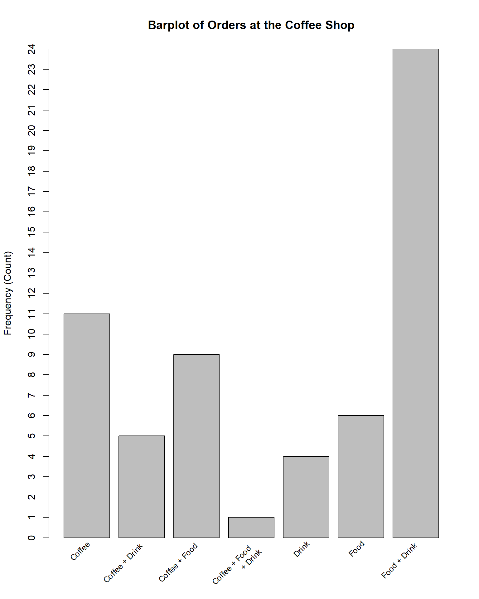
Example 11.2 (Charles and Sadie Count Coffee Orders, Representatively) With the understanding of the flawed methodology that they exhibited on their first attempt, Charles and Sadie decide to perform a random sample to collect data on the different coffee orders made at the local coffee shop. To this end, they randomly select different days of the week, different hours of the day, and then they observe all of the orders that come in over that time. Sadie produces the following bar plot based on their collected data.

Based on this plot, answer the following questions.

1. Which is the most common order in the sample, and what is the frequency with which it is ordered?
2. If there are a total of \(60\) orders, what is the relative frequency of the least common order?
3. How many orders had any coffee drink in the order?
4. Describe the overall frequency distribution.

Solution

1. In this sample, there are \(24\) orders of Food + Drink, which is the most common order.
2. The least common order is a coffee + food + drink, which occurred \(\dfrac{1}{60} = 0.01666\) proportion of the time in the sample.
3. In total there were \(11 + 5 + 9 + 1 = 26\) orders with coffee in them. This accounts for \(\dfrac{26}{60} = 0.433333\) of all orders.
4. The most common order was food and a non-coffee drink, which was more than twice as common as the next most frequent order of just a coffee. It was very unlikely for people to get all three categories of item. People got coffee with food more frequently than food alone, drinks alone, or coffee with drinks.

Whenever we present a descriptive statistic, be that a numerical summary or a graphical summary, it is always worth asking the question: “what are we trying to highlight?” In the case of frequency distributions, we are typically thinking about highlighting the total counts and cross category comparisons of the different values. Often times these are comparisons that we wish to make and using a bar chart for this is quite effective. However, depending on what we are trying to communicate, there may be alternative choices that make sense to make. It is always important to ensure that your visualization or summary is informed by the goal of your presentation, rather than by outside guidance. Descriptive statistics is fundamentally a field predicated upon communication. With that said, any time that we are presented with an observed qualitative variable, the frequency distribution completely contains all of the information in the data. It may not always be the most useful presentation of the data, however, it is a way of summarizing everything that we know about that variable alone. As a result, deep comfort with frequency distributions will be instrumental to effective communication and description of qualitative data.

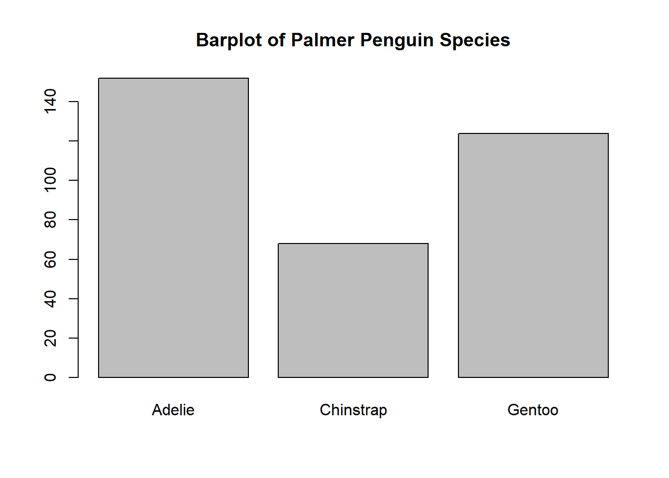
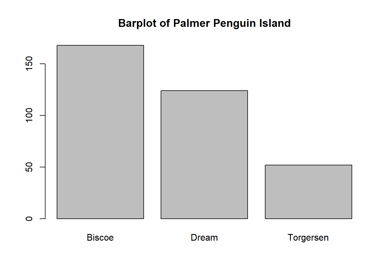
Example 11.3 (Charles finds Palmer’s Penguins) While daydreaming one day, Charles imagines the chance to work at the Palmer Station in Antarctica, researching penguins. The day dreams lead to a rich imagination, envisioning all species of penguins across the various islands. As the day dreams wind-on, Charles begins to count the penguins, leading to the following observations.

	Biscoe	Dream	Torgersen
Adelie	44	56	52
Chinstrap	0	68	0
Gentoo	124	0	0

Using these data⁸ answer the following.

1. Write down the complete frequency distribution for penguin species.
2. Write down the complete frequency distribution for the inhabited island.
3. Describe or sketch the bar plots for each of the relevant frequency distributions.

Solution

1. To get the distribution for species, we add up along each row to get the total observed data into a frequency table. To get the relative frequency, the frequency is divided by \(344\).

	Frequency	Relative Frequency
Adelie	152	0.4418605
Chinstrap	68	0.1976744
Gentoo	124	0.3604651

2. To get the distribution for locations, we add up along each column to get the total observed data into a frequency table.

	Frequency	Relative Frequency
Biscoe	168	0.4883721
Dream	124	0.3604651
Torgersen	52	0.1511628

3. The following represent the two bar plots for each distribution.

11.3 Descriptive Statistics for Quantitative Variables

Where our approach for qualitative data was to first summarize the data numerically, and then analyze, with quantitative data the first step is unnecessary. When our data are numeric to begin, we can work directly with them in order to begin to summarize the behaviour of the observed variables. Despite this change in process, the frequency distribution remains an impactful concept in summarizing and describing data which have been observed.

11.3.1 The Frequency Distribution for Quantitative Variables

If the quantitative variables that have been observed are discrete, the frequency distribution can proceed in an exactly equivalent way as in the qualitative case. If, however, we have quantitative variables our frequency distribution needs to be adjusted. The issue is that, if a variable of interest is continuous, we do not expect to ever observe the same value more than once. This renders the frequency distribution to look something like a broken comb⁹, rather than having any interesting features. To avoid this happening, we consider the process of binning quantitative variables, where values are placed into bins or classes, consisting of intervals, in order to better understand the structure of the frequency distribution.

Definition 11.2 (Data Binning) Data binning is a (pre-processing) step of a data analysis in which quantitative variables (typically continuous ones) are placed into bins or classes based on their underlying value. If a quantitative variable \(x\) takes values in the interval \([a,b]\), then the interval \([a,b]\) is divided into several sub-intervals, say \([a,p_1], [p_1, p_2], \dots, [p_{k-1},b]\). Then, each observed value for \(x\), \(x_i\) is placed into its corresponding bin, before the data are analyzed.

As a general rule, bins should be selected either based on some subject-matter justification (such that they are meaningful to the underlying data), or else to accurately balance the trade-offs of smoothness and accuracy in the frequency distribution. That is, we want to select enough bins so that the true behaviour of the data are correctly represented, while not selecting so many that noise and variability are the primary conclusions to be drawn from the summaries. Plenty of methods to select the number of bins have been proposed, and in most software packages for devising frequency distributions various techniques will be implemented. It is worth ensuring that the technique selected for any particular use case accurately summarizes and describes the available data. Generally, \(10-30\) bins will likely suffice, though fewer or more may be necessary in certain situations.

The only hard-and-fast rules of binning is that, first, bins should¹⁰ be of equal width. That is, if you take \([0,1)\) to be the first bin in your data, then every bin should be of length \(1\). Second, bins should¹¹ span the complete range of your observed data. If you have points ranging from \(0\) to \(1000\), every value between \(0\) and \(1000\) should be contained in some bin. Once binned, quantitative frequency distributions can be described in exactly the same manner that qualitative were.

Example 11.4 (Charles and Sadie Count Coffee Order Items) After their success in understanding the makeup of different coffee orders, Charles and Sadie set their sights on understanding the quantity of items ordered by customers at the coffee shop. The observe customers for an hour and consider the total number of items each customer orders. The following observations are made.

• 3
• 1
• 4

• 2
• 1
• 1

• 1
• 6
• 2

• 3
• 1

• 2
• 1

• 3
• 2

Based on these data, answer the following questions.

1. Write down the frequency distribution for the number of items on each order. Include the relative frequency for each observation.
2. Is data binning required for this frequency distribution? Describe.

Solution

1. Here the relevant categories are \(\{1,2,3,4,5,6\}\). We get

Order Size	Frequency (Count)	Relative Frequency
1	\(6\)	\(6/15 = 0.4\)
2	\(4\)	\(4/15 = 0.266666\)
3	\(3\)	\(3/15 = 0.333333\)
4	\(1\)	\(1/15 = 0.066666\)
5	\(0\)	\(0/15 = 0\)
6	\(1\)	\(1/15 = 0.066666\)

2. No. These data are discrete, and given that there are only \(6\) total categories there would be no particular utility to binning here. If the data were continuous, or were discrete with sufficiently many categories so as to be better treated as continuous than discrete, then binning would be pertinent.

Example 11.5 (Charles and Sadie Count Coffee Order Values) As a final way of understanding the distribution of different coffee orders, Charles and Sadie decide to observe the total cost of orders for various customers coming through the store. The following observations are made over the course of an hour.

• $2.25
• $2.20
• $5.13

• $1.30
• $2.02
• $4.91

• $1.64
• $3.49
• $0.98

• $2.97
• $3.84

• $5.30
• $2.53

• $2.45
• $4.66

Based on these data, answer the following questions.

1. Describe the considerations that should be made for bin sizes. Would a bin size of \(\$0.10\) be reasonable? What about one that is \(\$3.00\)?
2. Suppose that a bin size of \(\$0.50\) is used, starting at \(0.50\). Write down the frequency distribution.

Solution

1. The smallest observed value is \(0.98\) and the largest observed value is \(5.30\). That means that our bins should encapsulate both of these end points, and be evenly spaced throughout. Because there are only \(15\) data points, we likely want fewer bins rather than more, to ensure that our bins are not predominantly empty or with single items. If we use \(0.10\), we would require \(43\) bins at least to include all of the data. This would guarantee that most bins were empty, and is far too small of a divide to be useful. If we used \(\$3.00\), we would span the full range in \(2\) to \(3\) bins. This is likely not particularly informative either, this time giving too little of a breakdown of the various values.
2. The following is the relevant frequency distribution.

Bin	Frequency (Count)	Relative Frequency
\([0.50,1.00)\)	\(1\)	\(1/15 = 0.066666666\)
\([1.00,1.50)\)	\(1\)	\(1/15 = 0.066666666\)
\([1.50,2.00)\)	\(1\)	\(1/15 = 0.066666666\)
\([2.00,2.50)\)	\(4\)	\(4/15 = 0.266666666\)
\([2.50,3.00)\)	\(2\)	\(2/15 = 0.133333333\)
\([3.00,3.50)\)	\(1\)	\(1/15 = 0.066666666\)
\([3.50,4.00)\)	\(1\)	\(1/15 = 0.066666666\)
\([4.00,4.50)\)	\(0\)	\(0/15 = 0\)
\([4.50,5.00)\)	\(2\)	\(2/15 = 0.0.1333333\)
\([5.00,5.50)\)	\(2\)	\(2/15 = 0.0.1333333\)

While the tabular representation of the frequency distribution for quantitative variables is a relevant summary, and one which serves a key role, we will see that there are far more ways of summarizing the behaviour of quantitative variables. Before that, however, it is worth determining how to graphically represent a quantitative frequency distribution, through the use of histograms.

11.3.2 Using Histograms for Visualizing Quantitative Frequency Distributions

If we expand the idea of a barplot to quantitative variables, we get the histogram. A histogram is primarily useful for displaying the distribution of a single quantitative variable. To do so, the horizontal (x-axis) represents the value of the variable of interest, and the corresponding vertical (y-axis) represents the frequency with which that value occurs in the data. That is, higher points correspond to more frequently occurring values, and lower points correspond to less frequently occurring values.

If the data are binned, then the histogram displays counts within the bins rather than at the values themselves. Just as with a barplot, the graphic proceeds by drawing a rectangle, with a height equal to the frequency, and a width equal to the length of the interval. The larger the rectangle, the more points that were observed in that range.

Sometimes, instead of having the y-axis measure the frequency, we may take it to measure the density of falling in that range. The density is given by the probability that a value in that range is observed, divided by the width of the range. For instance, if \(10\) of \(50\) observations fell between \(2\) and \(4\), then the height of the rectangle using the density representation would be \(\dfrac{10/50}{4-2} = 0.1\). So long as every bin has an equal width, the same relative heights will occur whether using the frequency or density versions.

A key difference between histograms and barplots is that, since the data in a histogram are numeric, we typically consider the x-axis to be continuous. This means that the bins of the histograms expand along the complete axis, and adjacent bins will touch one another. In a barplot there is separation between these categories since there are no values between the two of them.

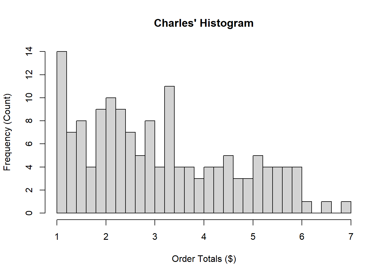
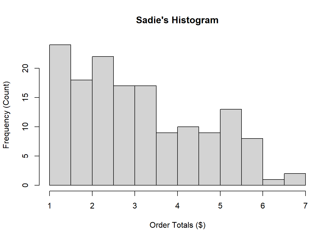
Example 11.6 (Charles and Sadie Plot the Coffee Orders) Charles and Sadie realize that to make sure that they have a full understanding of the total spend that customers have at the coffee shop they should likely collect more data, and data which are spread out randomly over times of the day and days of the week. As a result, they conduct another random survey. Once collected, both Charles and Sadie produce histograms for the totals, as seen here.

1. What is the approximate bin width used by Charles? By Sadie?
2. Describe the frequency distribution as depicted by both histograms.
3. Does one histogram do a better job than the other at representing these data? Explain.

Solution

1. We can see that in every dollar along the x-axis, Sadie has two histogram rectangles. This suggests a bin width of approximately \(0.50\). For Charles, there are \(5\) per dollar, and as a result, the bin width will be approximately \(0.20\).
2. Both plots demonstrate that the most frequent order totals are comparatively low, with values around \(\$1.00\). With the histogram provided by Sadie, the order totals are fairly uniform between \(1\) and \(3.50\), with a small spike around \(2.00\). Following that, the order totals are fairly uniform between \(3.50\) and \(6\), before falling again above \(6.00\). The patterns in the histogram from Charles are similar, but with slightly more information. While there is a fairly uniform distribution of observations beyond \(3.40\), and then a dip beyond \(6.00\), for the smaller values there is an oscillating pattern. They spike around \(1.00\), \(2.00\), \(3.00\), and \(3.40\), with the other values being appreciably lower. Still, the lower values are definitely higher on average than the higher values, with roughly equivalent breakpoints as was seen with Sadie’s.
3. The preferred histogram here will likely depend on the use case for the data. The data that Charles is demonstrating provides more specific information, however, it is possible that this added information is more noise than useful. It would be interesting to look at, for instance, the prices of various items at the store to see if there was a reason for the peaks: otherwise, it could be seen to be random variation that is not particularly noisy. Sadie’s pattern, by contrast, is far more explicable, but it gains this by smoothing over a lot of the fine details within the graphic. Perhaps a graph that balances these two would be more suitable.

A histogram is a useful graphical display since it succinctly summarizes the entire distribution of a particular variable. You can easily see the range of the data, the points which came up frequently in your observations, those which were rare, and how this behaviour is expressed throughout. It will allow you to readily view points that appear to not fit the trend of the rest of your data, and to investigate a single variable at a glance.

When constructing a histogram, the primary decision that needs to be made is how many bins you should use, or equivalently, how large your bins should be. As you have more and more observations you can typically get away with using smaller bin sizes as, even at the smaller sizes, you likely still have observations that fall into the given intervals. Just as with the discussion on data binning, software that implement histogram construction often provide several techniques for choosing a bin size, or the number of bins, in order to best summarize the data. It is worth considering these for the problem at hand, and ensuring that the choice that is made illustrates the data faithfully.

11.3.3 Characteristics of the Frequency Distribution

While we will typically focus on graphically displaying the distribution of a dataset, it is useful to consider what it is specifically that we are trying to display, and what are the properties of a dataset which are of interest to us? We are primarily concerned with three properties of a distribution: the location, the spread, and the skewness. We have seen all three of these concepts when discussing random variables, but their importance becomes central when summarizing data. More concretely, when describing data we want to make sure to describe the shape of the distribution, the centre of the distribution, and the spread of a distribution. Each of these three concepts have different measures or components which, when taken together, serve as a more complete description of the frequency distribution.

Definition 11.3 (Shape (of a Distribution)) The shape of the data distribution refers to the general pattern of points that are observed in the specific dataset. Typically, the shape of a distribution is decomposed into the modality and skewness of the distribution.

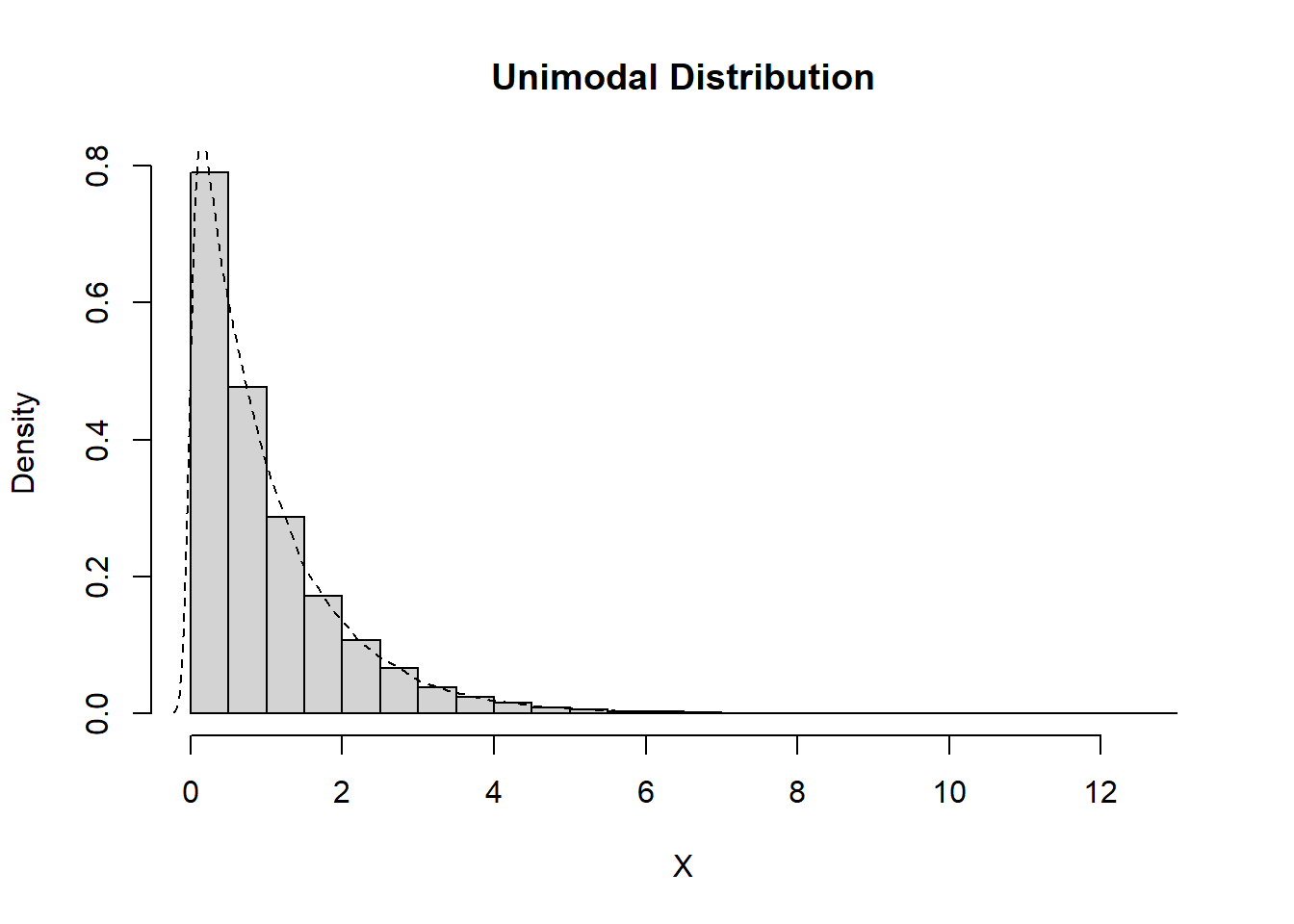
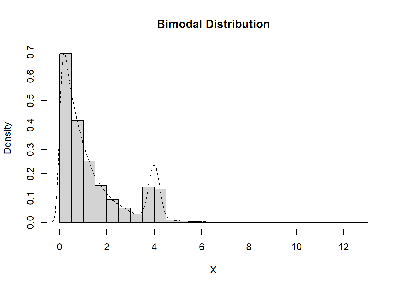
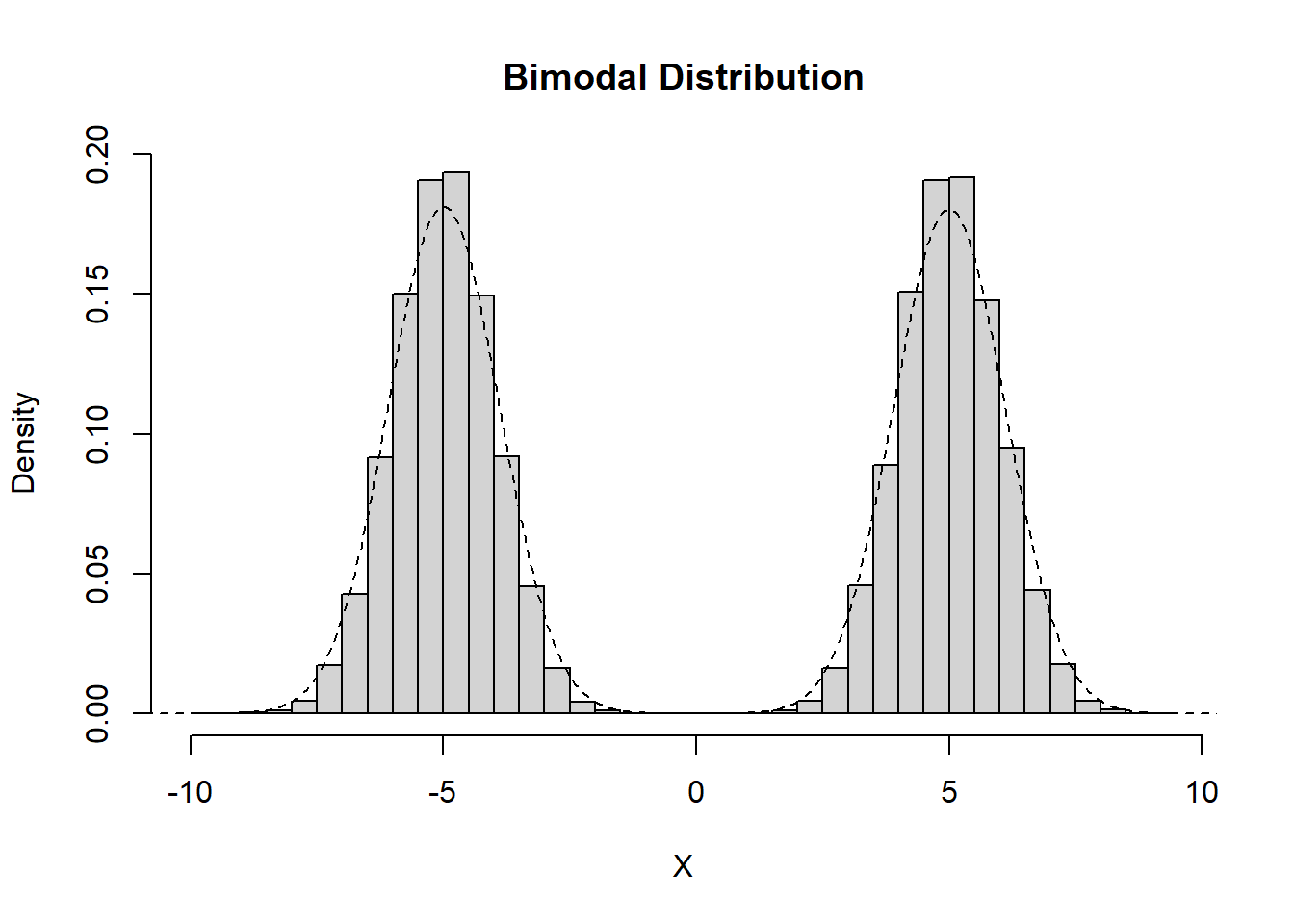
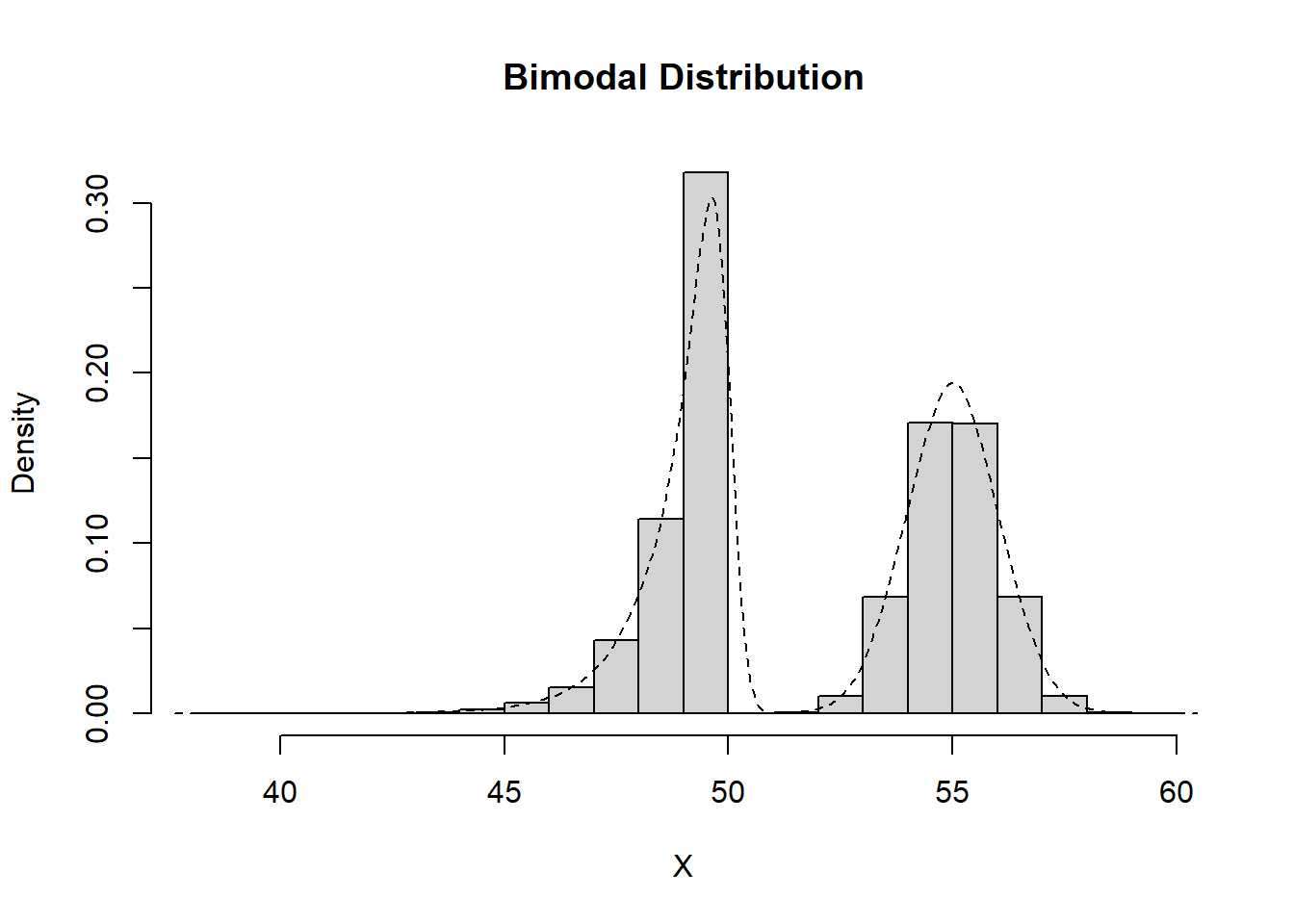
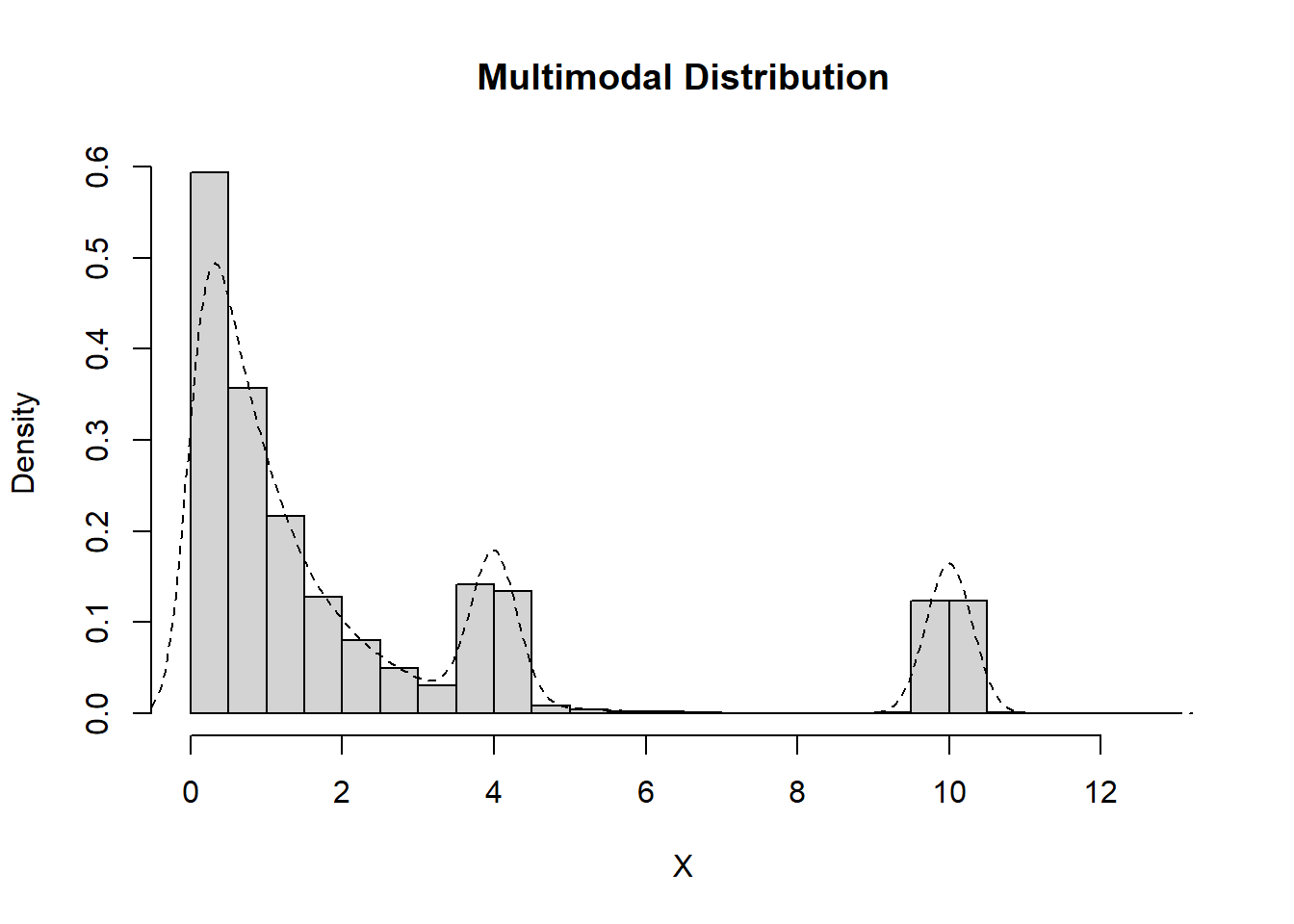
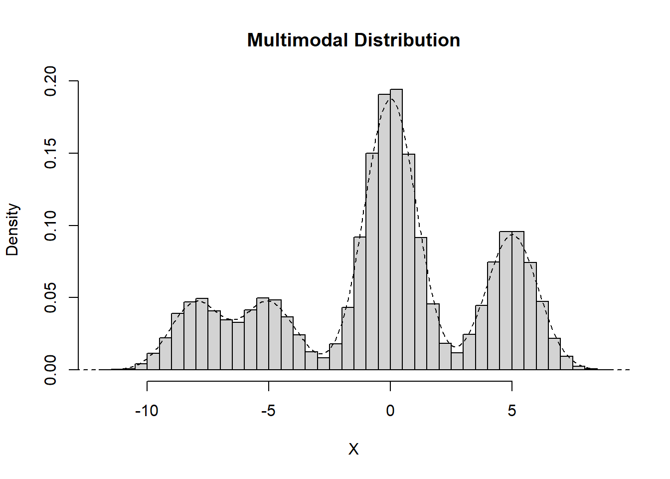
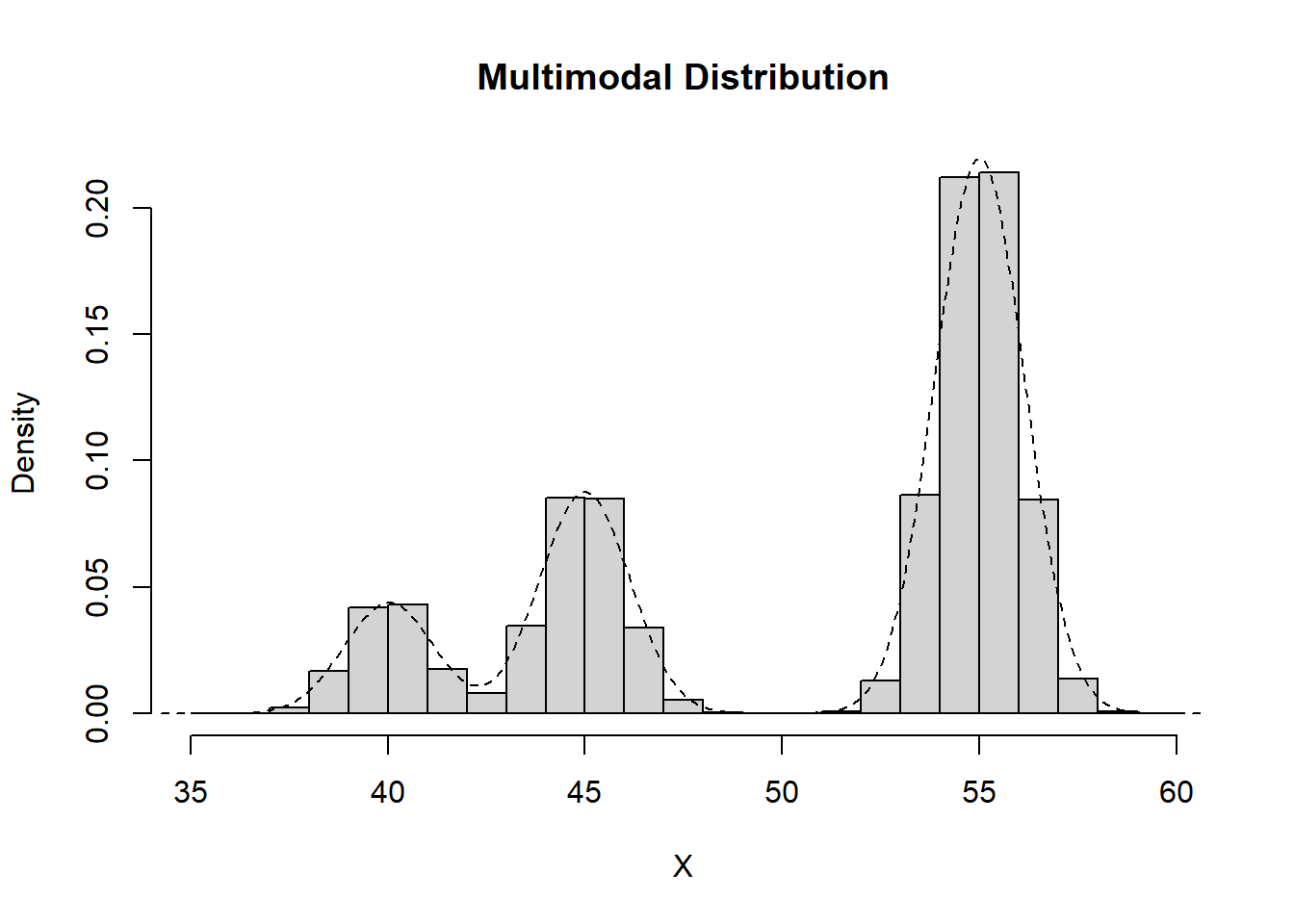
The modality refers to the number of peaks that are visible in the distribution: points that are higher than the surrounding points. A distribution is unimodal with one peak, bimodal with two peaks, or multimodal with more than two.

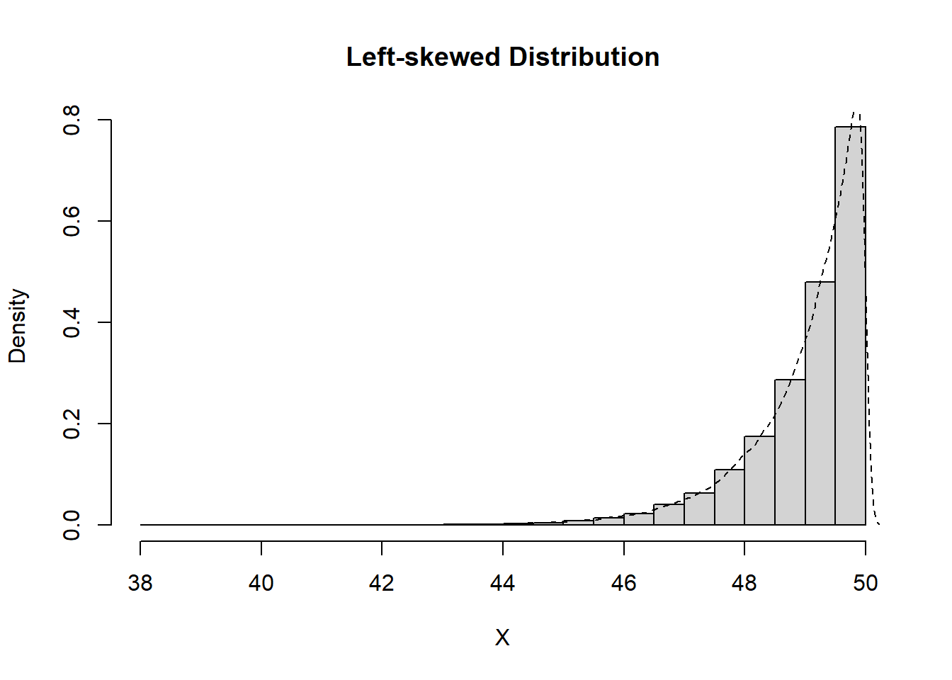
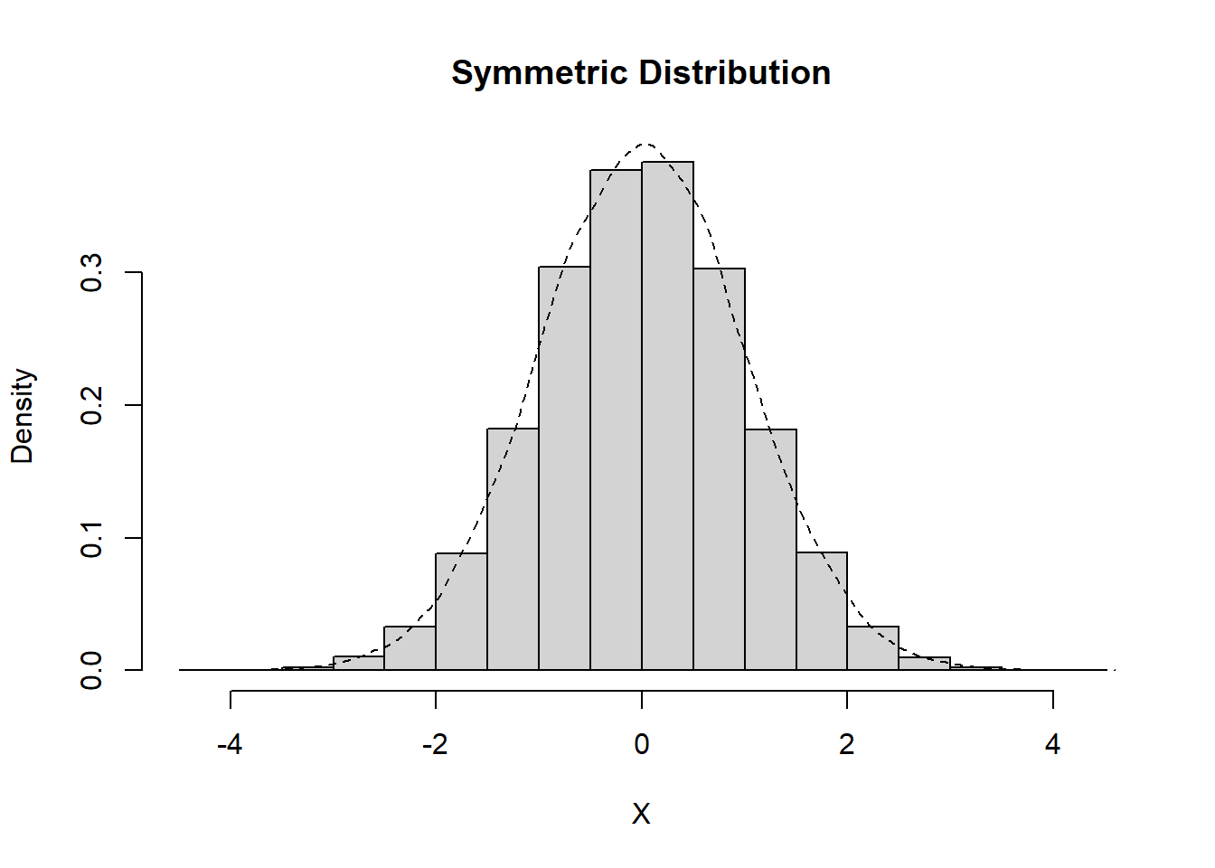
The skewness corresponds to how symmetric (or not) a distribution is. If a distribution can be mirrored around its center, with the same behaviour above and below the central point, we describe it as symmetric. If a distribution has differing tail-behaviour, extending out in a direction, we say that it is skewed. A distribution that has a long-tail to the right is called right skewed or positive skewed, where a distribution that has a long-tail to the left is called left skewed or negative skewed.

To describe the shape of a frequency distribution, we describe the modality and the skewness of it. These two features combine to give a good sense of the general picture of the distribution, such that someone should be able to sketch a reasonable approximation to the frequency distribution from the description. However, there are many distributions with the same modality and skewness, which are otherwise quite distinct. To understand these differences, it is useful to turn towards measures of location, or central tendency, and measures of spread, or variability.

Definition 11.4 (Location (Central Tendency)) The location of data, also referred to as the central tendency, is a description of where observations in the dataset tended to fall around. This can be measured as the sample mode, the sample median, or the sample mean, and is typically summarized using all three. Measures of central tendency give a sense as to where the middle of the data were, where various definitions of middle can be used.

Just as with random variables, measures of location come about by asking what we “expect” to see in the data. When we are discussing samples, rather than random variables, we are instead answering questions around what we saw on average, or what we tended to see in the observed data. Location summaries are quite common, and quite intuitive. You may indicate the most common value, which is the sample mode, or the overall average, the sample mean. However, just as with random variables, the measures of central tendency only tell a partial story. The other key feature of the data is the spread.

Definition 11.5 (Spread (Variability)) The spread of data is a measure of how separated the data are, and how they tend to be spaced around the location. The spread can be captured using particular measurements, such as the sample variance, sample IQR, or sample range as was done with random variables. The may also refer to the tail behaviour of the data, which looks at how likely values are as they move further and further from the center of the data.

A distribution is said to be heavy-tailed if points that are far from the measures of central tendency are quite frequent in the data, and is said to be light-tailed otherwise. These concepts can be formalized more rigorously, however, it is often taken to be an informal rather than formal check.¹²

The spread of the data gives a measure as to how concentrated (or not) the observations were. Data which are widely spread out will have large measures of variability compared to those which are less spread out. When combined with the measures of central tendency, as well as a description of the shape of the distribution, it is possible to develop a fairly clear picture of the behaviour of the data, summarized rather succinctly.

11.3.4 The Shape of a Distribution

As indicated, the shape of a distribution is primarily defined by the modality and skewness of the distribution. That is to say, when asked to describe the shape of the distribution, you should report on the modality (including the values of the modal points), as well as on the symmetry or skewness of the distribution.

Definition 11.6 (Modality) Modality refers to the number of local peaks that a frequency distribution has. That is, the number of times that there are values in the frequency distribution that are higher than those in close proximity to them. If looking at the histogram we are looking for the number of “hills” that exist. Modality is classified by the number, and values, of the different modal points.

A distribution with one local maximum is considered unimodal. A distribution with two local maxima is considered bimodal. A distribution with three or more local maxima is considered multimodal.

It is important to emphasize that a frequency distribution may have only one mode, but may be multimodal. That is, we do not require each of the peaks to tend to equate to exactly the same level to be considered peaks. Instead, we compare them to only the points that are around them. This way, we can capture the idea of local behaviour indicating that certain regions appeared more frequently than others around them, which is often of direct interest to us. It is also important to recognize that, if reading modal points from a histogram, the number of breaks and the number of observations will likely change the perception of the modality. There will often be judgment calls when discussing the number of modes that a histogram exhibits, with reasonable disagreement being possible. As a general rule, you should not consider small noisy peaks adjacent to others to be additional modal points, unless there is a good reason to do so. If you envision drawing a smooth line over the full distribution of data, the modal points will come where you draw the crests of the hills.

Identifying the Modality of Distributions

Unimodal

Data which exhibit a single peak, whether this is in the center or off to one side, are considered to be unimodal.

Bimodal

Data which exhibit exactly two peaks are considered to be bimodal.

Multimodal

Data which exhibit more than two peaks are considered to be multimodal.

Beyond modality is the skewness. Skewness, or conversely, symmetry is a way of describing the tail behaviour of a distribution. As you move away from the central values, the most common values, or the middle values of a distribution, the tails are the values that are far from where you started but still present in the data. In general, if the tails going to the positive and negative directions look similar, the data are said to be symmetric. Otherwise, the data are said to be skewed. We differentiate skewness based on the direction that the tail travels.

Definition 11.7 (Skewness) Data which are nonsymmetric are said to be skewed. The lack of symmetry can be identified by the behaviour of the tails of a distribution, differentiating between positive (or right) skew and negative (or left) skew.

Data are right-skewed if the tail is longer to the righthand side of the figure. Data are left-skewed if the tail is longer to the lefthand side of the figure.

Sometimes skewness is quite dramatic, being very evident in which direction the skew will be. In other cases the data are not symmetric, but are also not evidently skewed. In these settings it is worth investigating the data in slightly more depth to try to understand whether the lack of symmetry (or skewness) can be explained based on some particular values, and if the remaining data exhibit a more predictable pattern.

Identifying the Skewness of a Distribution

To identify whether data are symmetric, right-skewed, or left-skewed, you consider the beahviour of the tails.

As a result, when asked to identify the shape of a distribution, you are being asked about the key features of the distribution: how many modal points are there, and where are those located, and what is happening with the tails of the distribution? Beyond these points, discussion of the shape of the distribution largely centers around giving added context to the nuance with the provided descriptors. For instance, if the skewness is not partiuclarly pronounced, that can be discussed. If modal points are not clearly delineated, that should be acknowledged. Once described, an individual should be able to sketch out a rough distributional curve that approximately mirrors the behaviour of the frequency distribution.

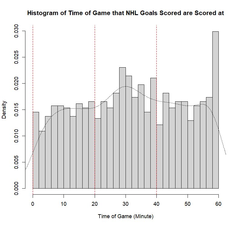
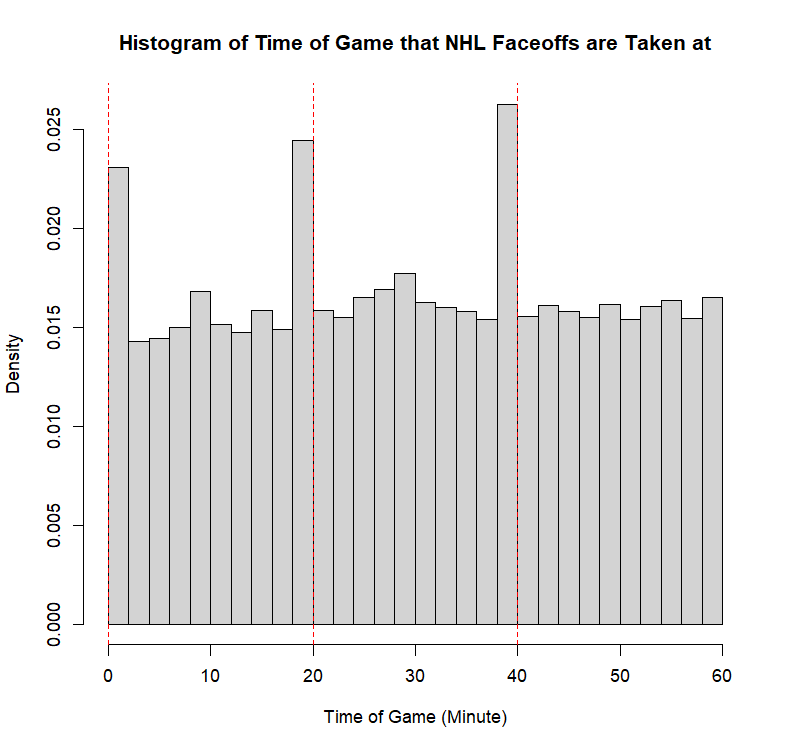
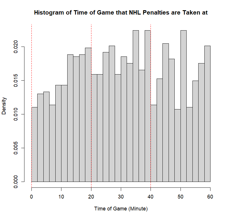
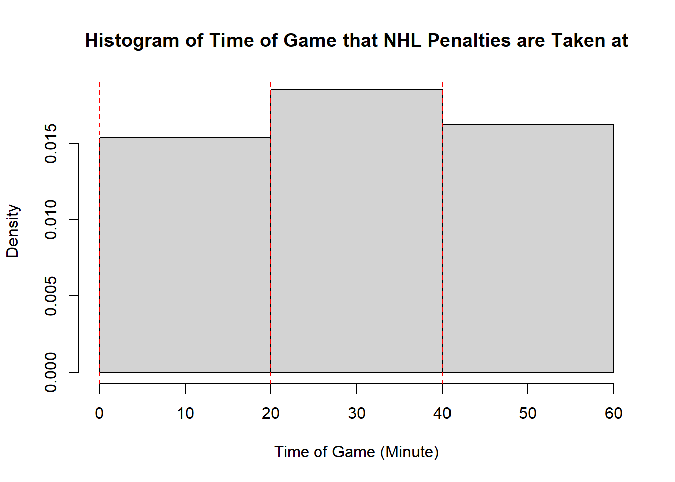
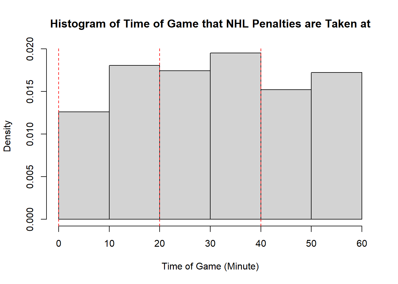
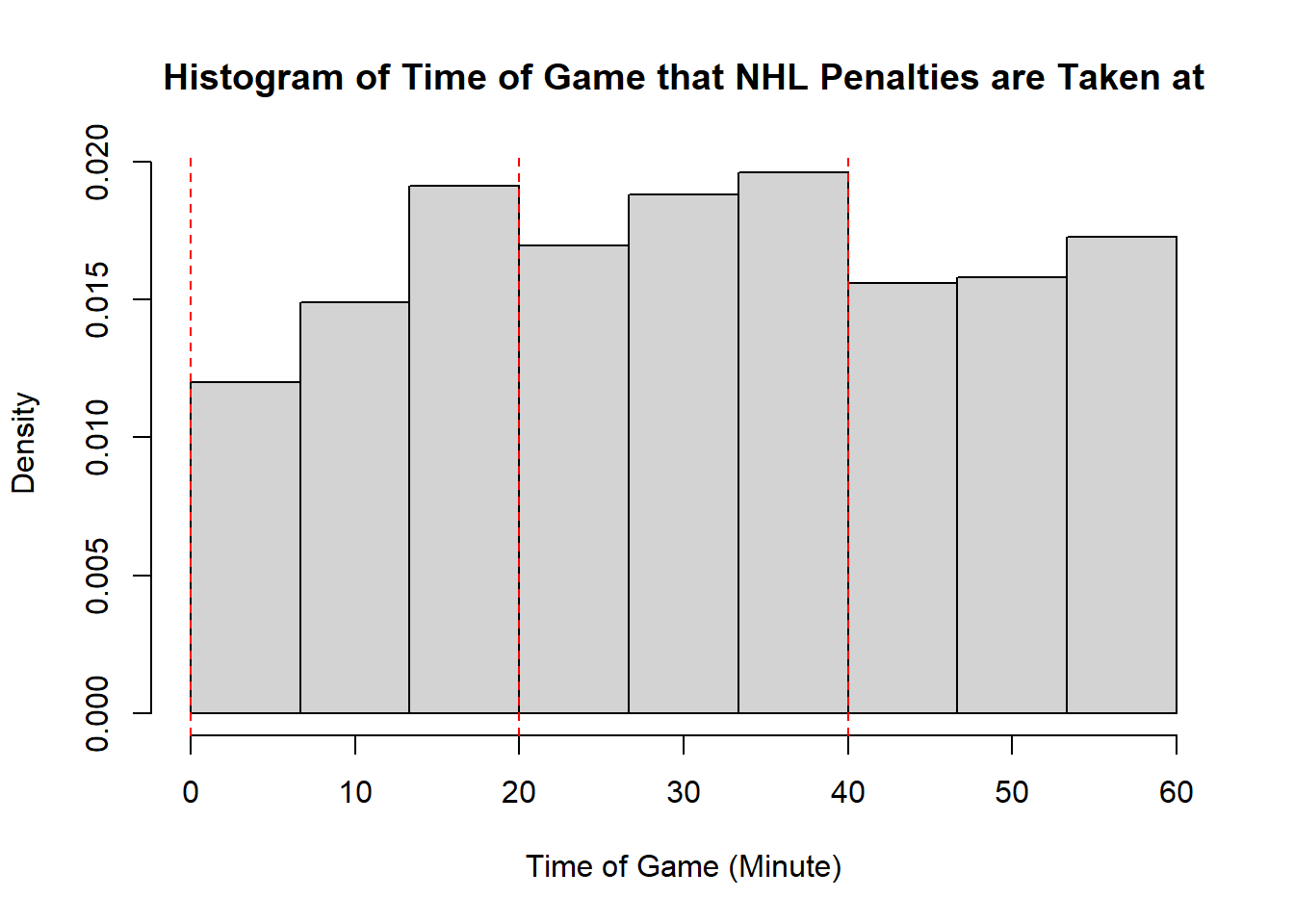
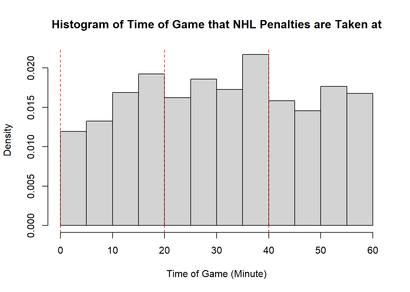
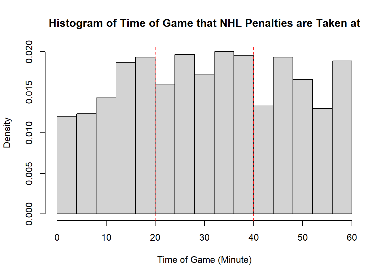
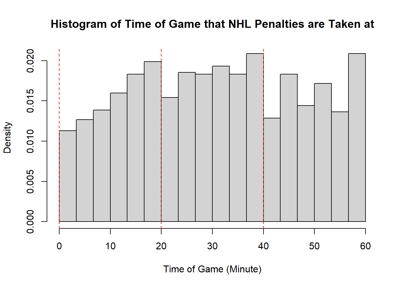
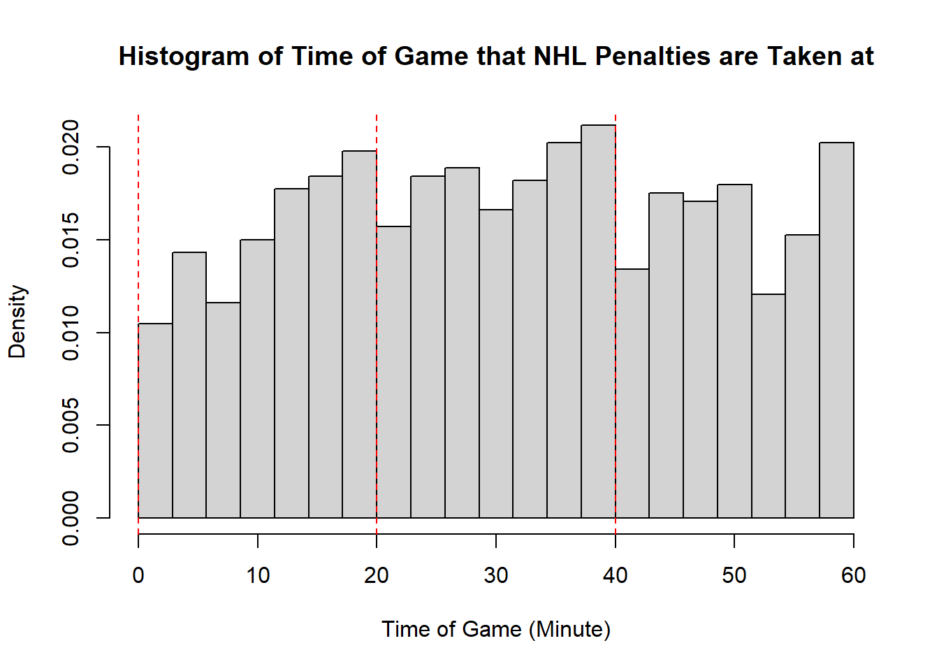
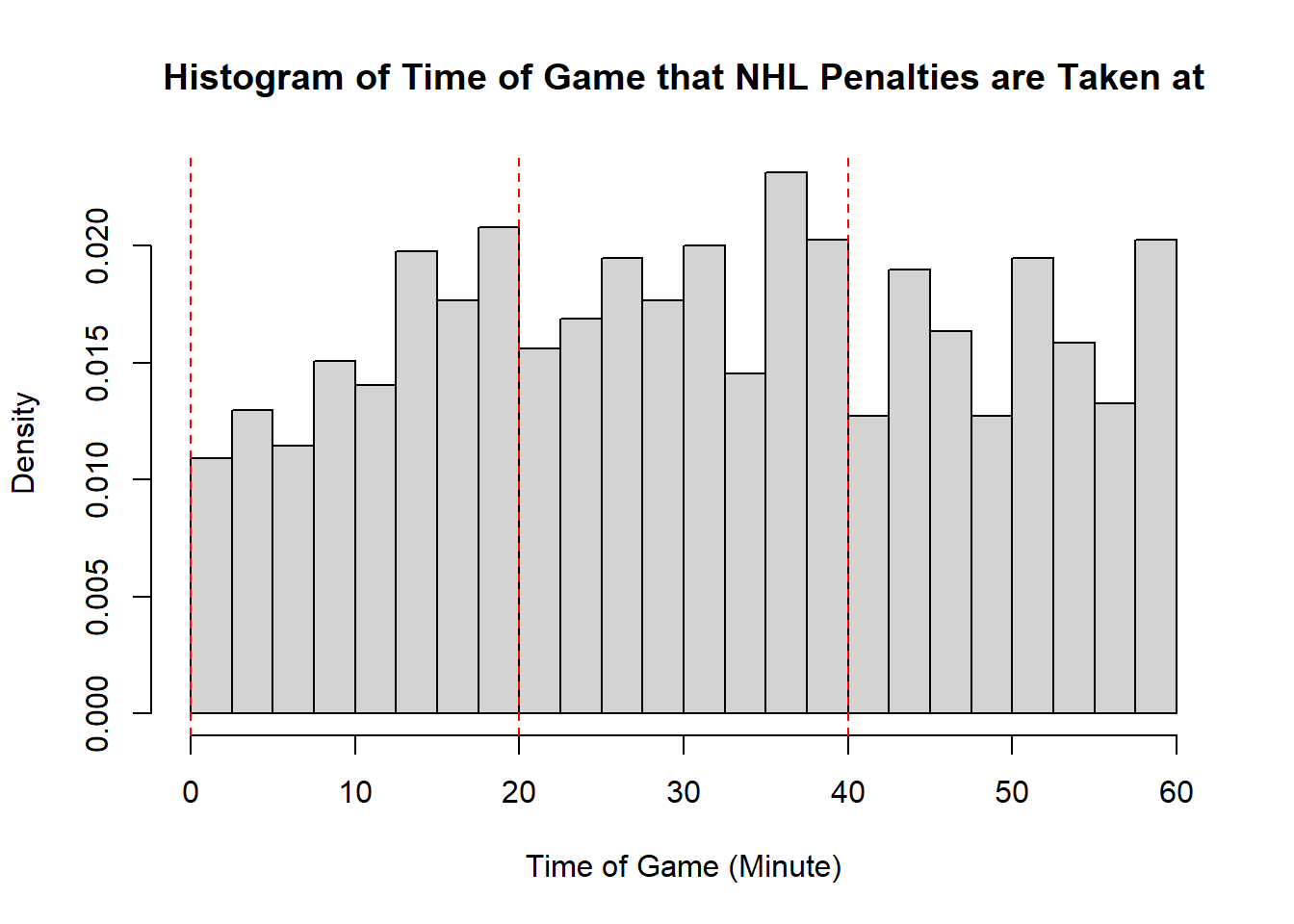
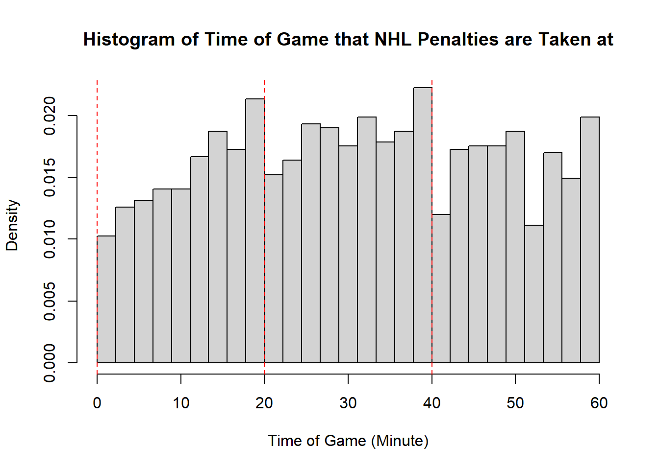
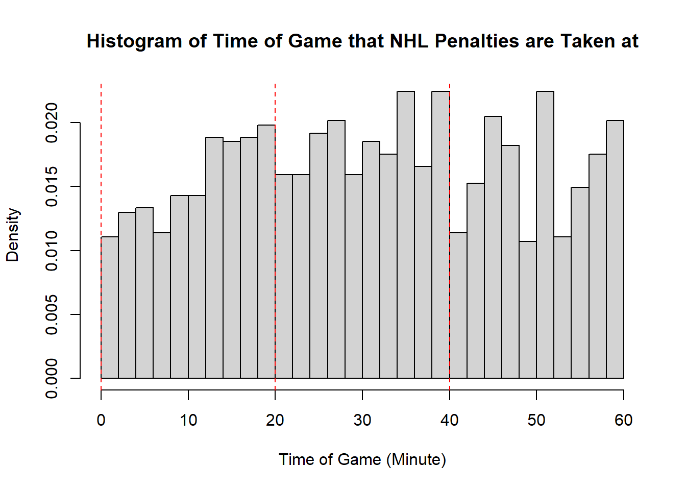
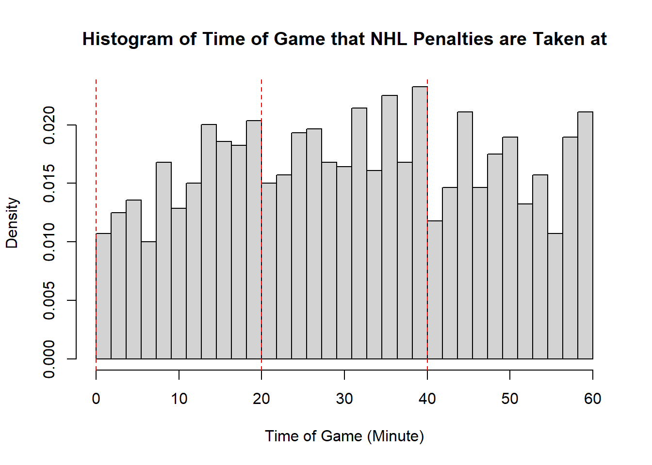
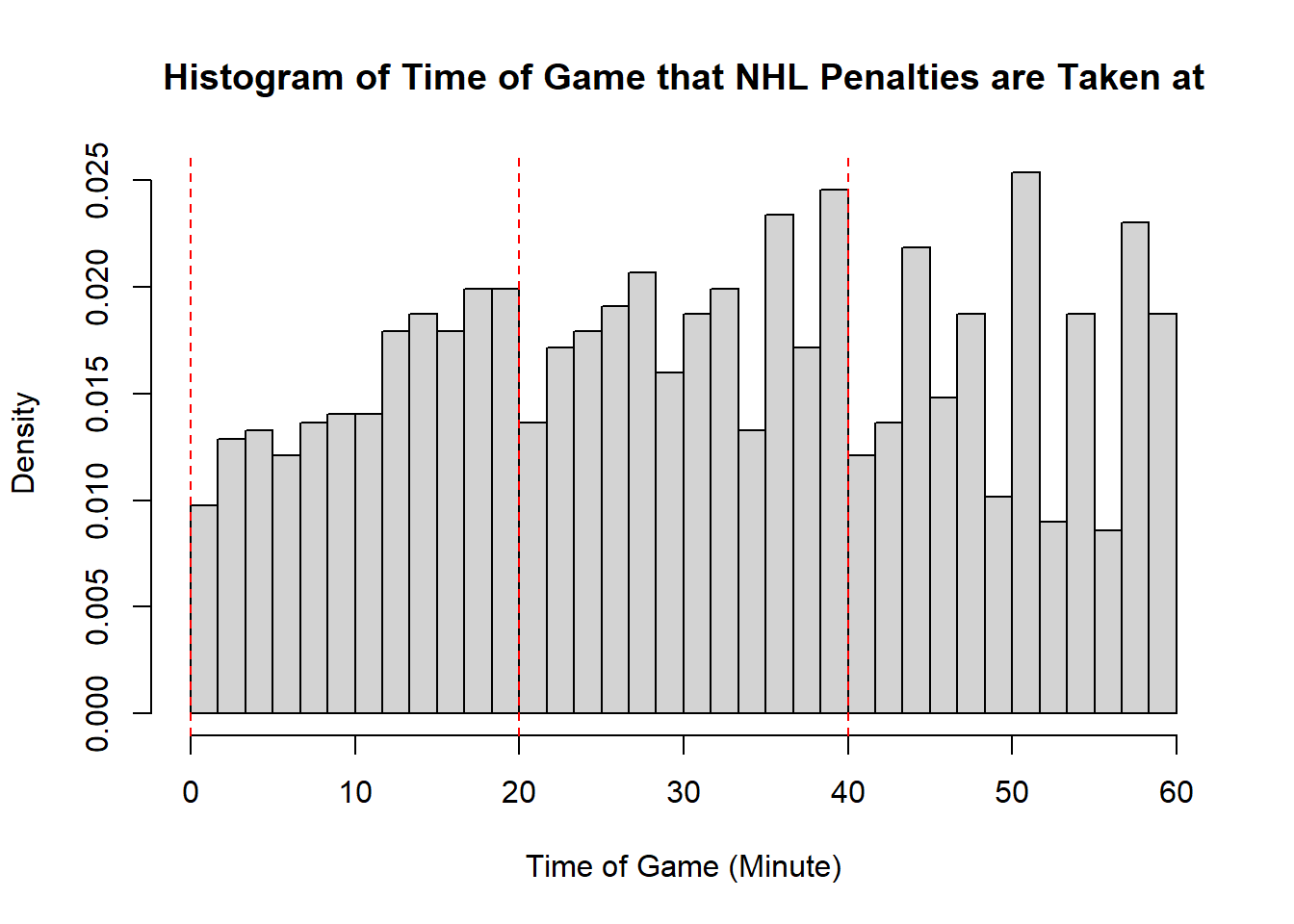
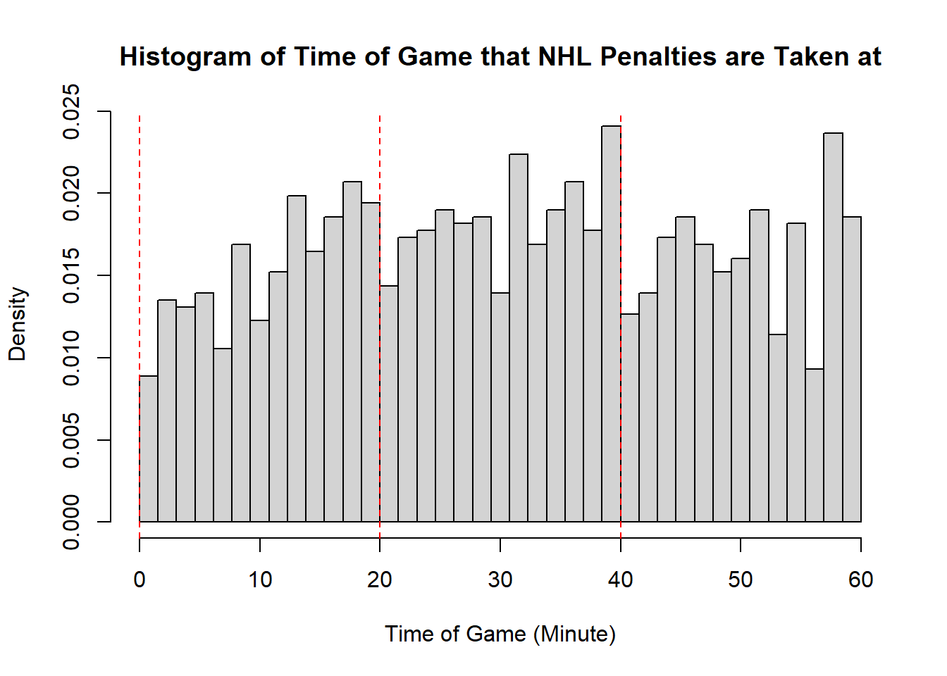
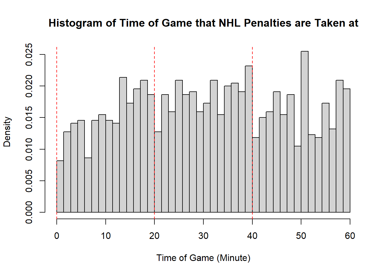
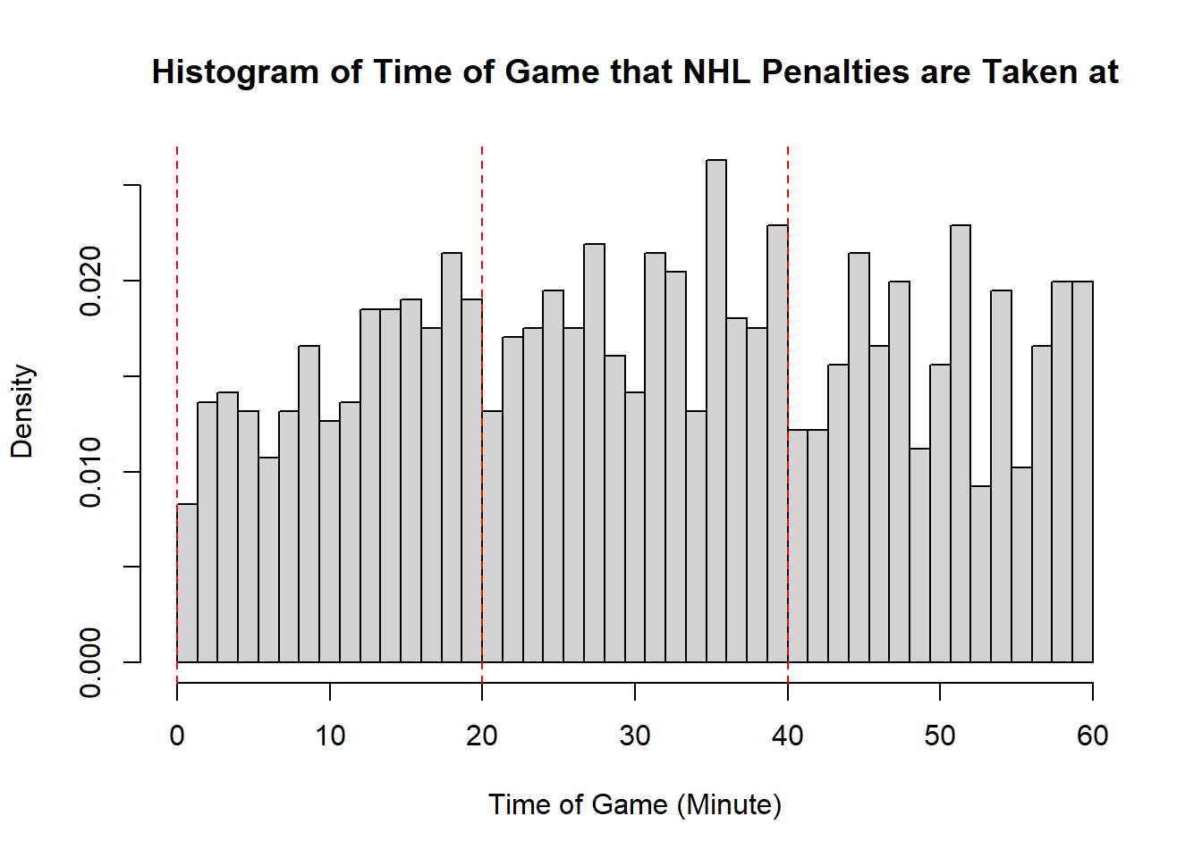
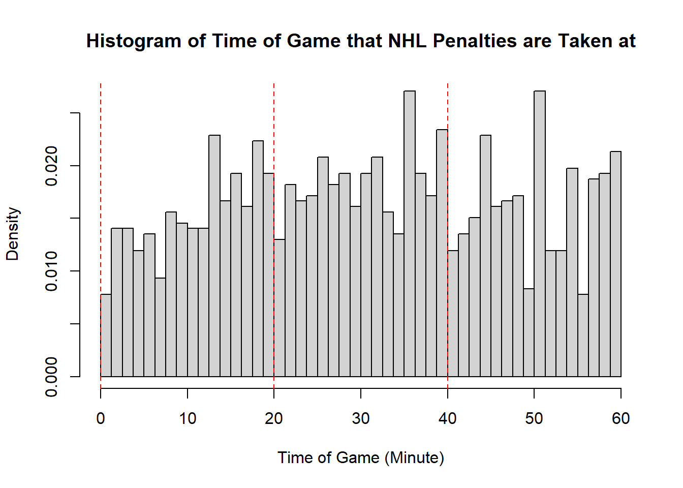
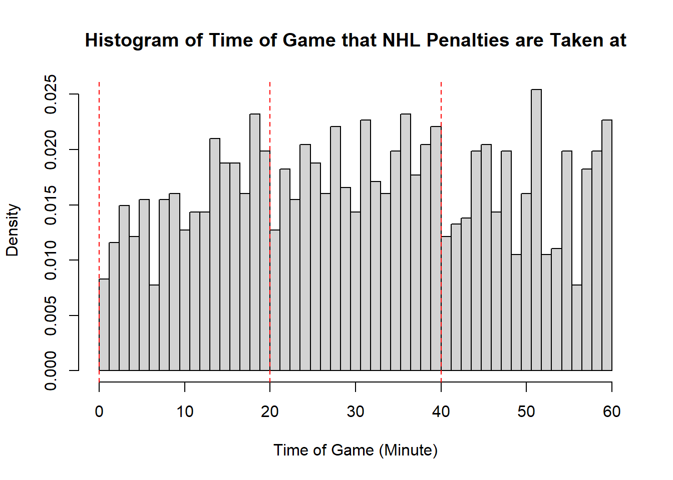
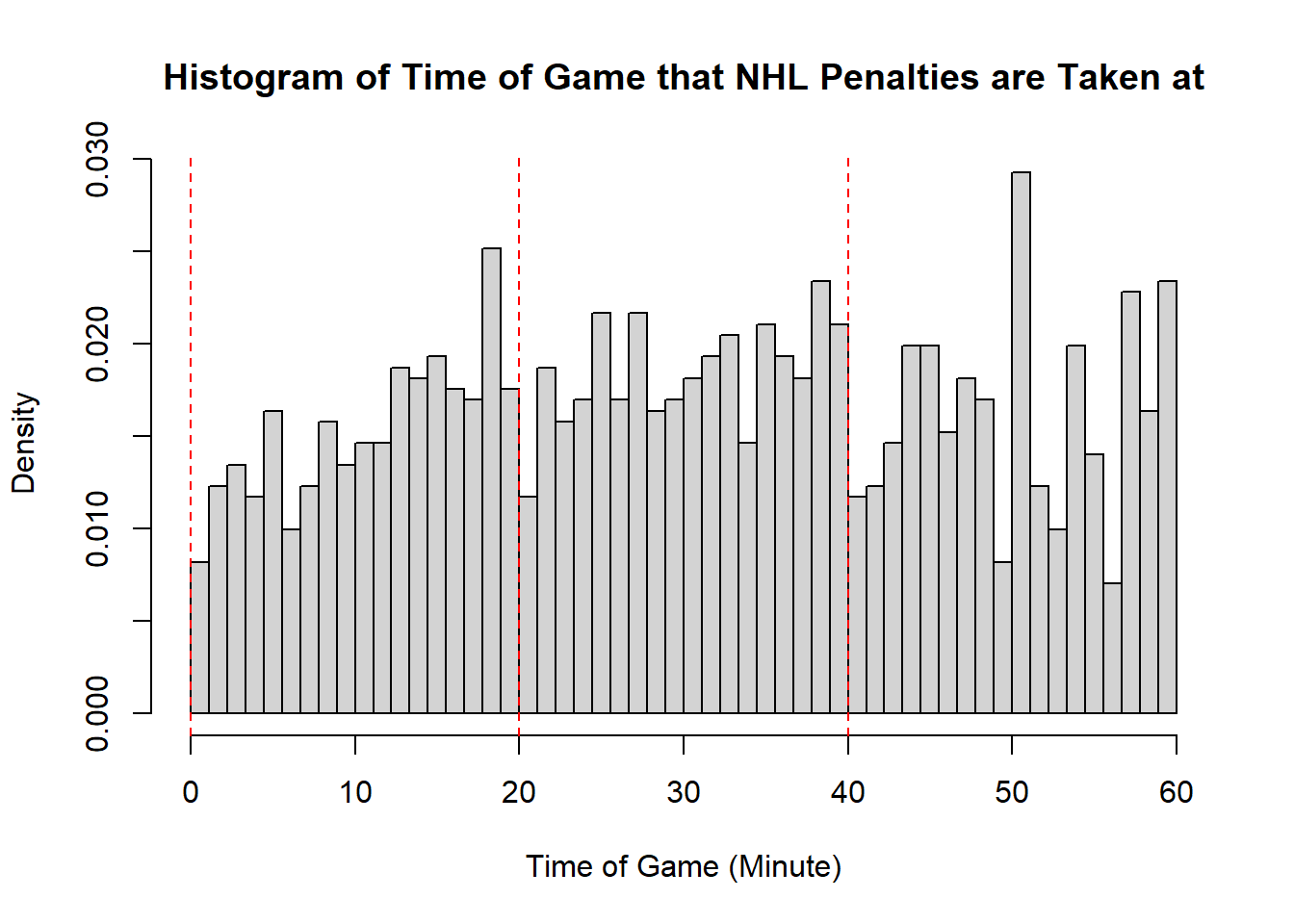
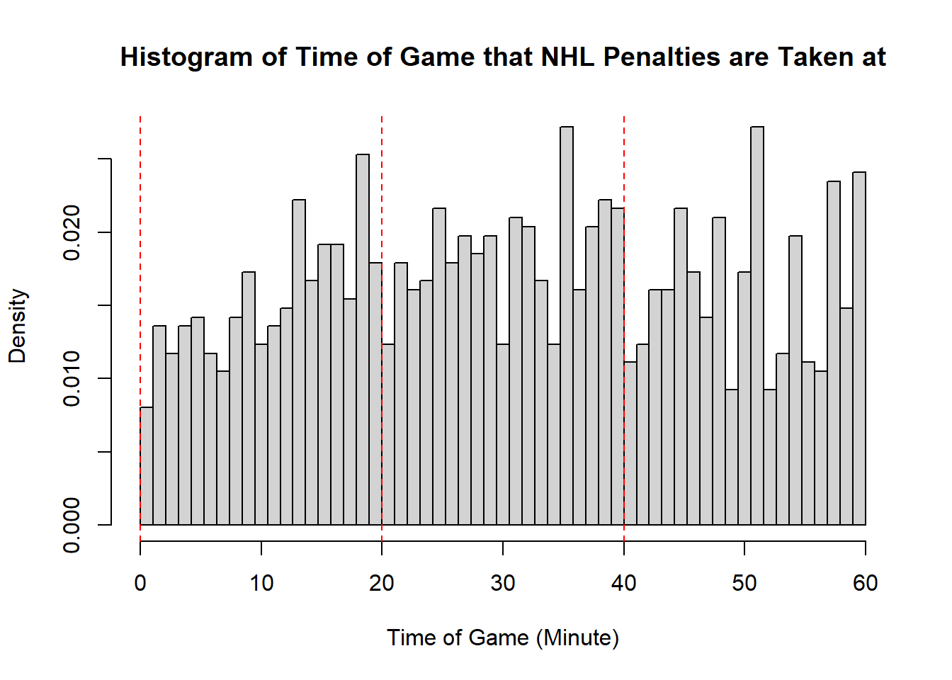
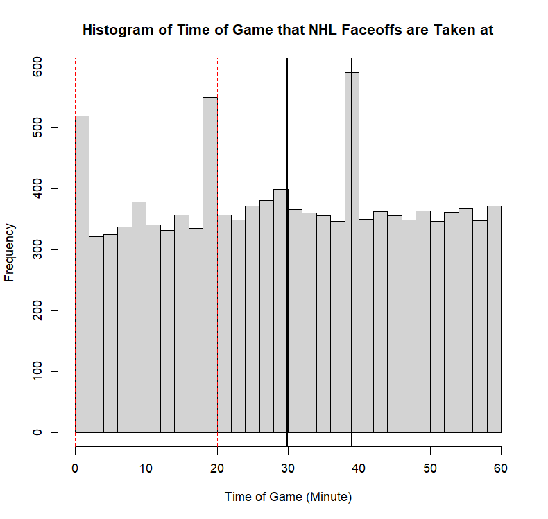
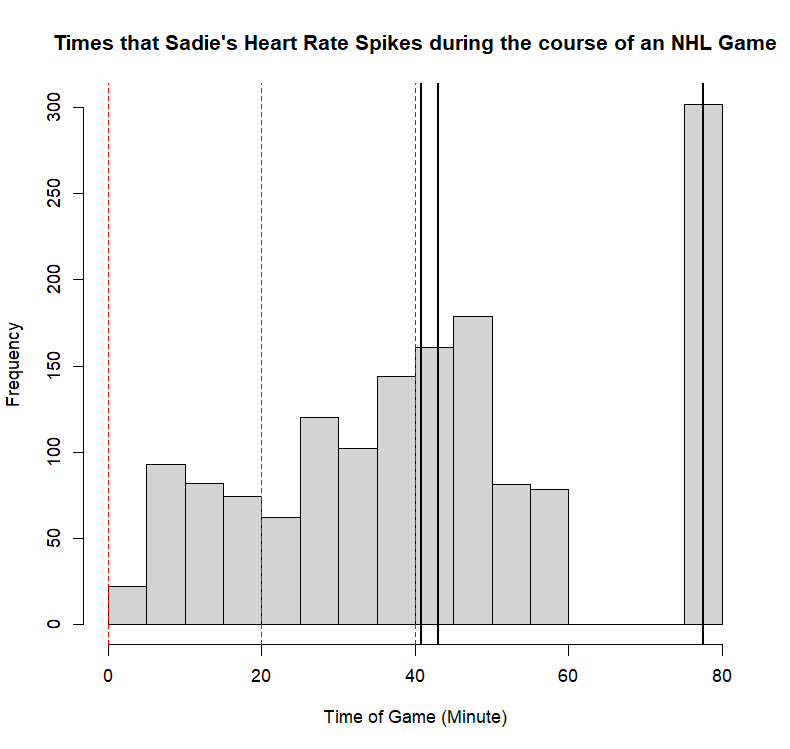
Example 11.7 (Sadie Records the Timing of Hockey Events) Sadie, being a big sports fan, has started to record and analyze the timing of different events throughout the game. Charles decides to help out by producing histograms for the time that these events happen at. Sadie records the time that faceoffs occur at, that goals are scored at, and when penalties are taken.¹³ The histograms are provided below.

1. Describe the shape of the distribution of goal times in NHL regular season games.
2. Describe the shape of the distribution of faceoff times in NHL regular season games.
3. Describe the shape of the distribution of penalty times in NHL regular season games.
4. Indicate any difficulties in describing these distributions.

Solution

1. The distribution is approximately bimodal, with modal points at approximately \(30\) and \(60\) minutes. The distribution is non-symmetric, since higher frequency of goals are scored near the end of the game than at the beginning, making it a left-skewed distribution. If the final bin is ignored, which may be reasonable given that the final minute of game has different dynamics than other times, the distribution appears roughly symmetric.
2. This distribution is approximately multimodal. The modes occur at \(0\), \(20\), and \(40\) minutes. Every period starts with a faceoff, and as a result, every game will have faceoffs taken at exactly \(0\), \(20\), and \(40\) minutes into it. There are some points which may be described as modal points around \(10\) minutes and around \(30\) minutes, but these are far less obvious than the other three. The distribution is non-symmetric owing to the lack of a modal point at \(60\) minutes. Because of this, we may say that there is a slight positive skew to the distribution. It seems more sensible, however, to indicate that in the absence of the three modal points that are clearly explicable, it is a roughly symmetric distribution that is approximately uniform across the whole range.
3. The modality of the penalty timings is difficult to describe. It may be reasonable to describe this as multimodal with modes appear around \(20\), \(25\), \(38\), \(45\), and \(60\). However, this may also represent some histogram noise that is better to smooth over. In that case, perhaps you suggest that the three modal points are around \(20\), and \(40\), and around \(50\). The distribution does not exhibit perfect symmetry, owing to the spike near the end of the games, however, there seems to be little apparent skewness in the distribution. With the points near the end of the game removed, it is a mostly symmetric plot, however, with those points in there is some negative skewness indicated.
4. While the first two distributions are fairly clear to describe in shape, the penalties are a lot less evident. This becomes even more apparent when we consider how the number of bins selected impacts the overall shape of the distribution. Consider the following histograms (if online, you can click to enlarge them). With few bins, this distribution appears to be approximately symmetric with a single mode in the middle of the distribution. As more and more are added, the pattern remains rather similar until a within-period distribution emerges: the first period has a negative skew, unimodal distribution, the second a fairly uniform symmetric distribution, and the third a bimodal negative skew distribution. As we continue to add bins we see histograms that look similar to the one we considered, before getting to a point that looks more or less consistent throughout the range, with seemingly random spikes at various times. These demonstrate the importance of bin size selection, and illustrate the challenges that can occur when trying to describe real-world data.

11.3.5 Measures of Location

The shape of a distribution is described in fairly general terms. If you know that a distribution is right-skewed and unimodal, with a peak around \(10\), there are many plausible distributions that could be drawn for what this would look like. While often times this shape captures the most pertinent information for a distribution, sometimes we require more. To add specificity, we can consider the location or central tendency of a frequency distribution. The main measures of location are the sample mean, sample median, and sample mode. These correspond to the exact quantities that we saw in random variables, this time computed on the data directly.

Definition 11.8 (Sample Mode) The sample mode is the most common value observed in a dataset. When there are more than one value which appear equally often, these are all consider modes. If a variable is binned, we may define the mode in terms of the classes rather than the specific value, depending on the context.

Whichever value appears most often is given as the mode. This is analogous to the most probable value for a random variable. The sample mode and the modal points are related to one another. When discussing modality, we contented ourselves with approximations, considering values near the actual modal points when defining the peaks. When discussing the sample mode we are looking for a specific value, or a specific category of values, which actually gives the most frequent value.

Definition 11.9 (Sample Median) The sample median is the middle point after ordering the observed data. If there are an even number of observations it is the mean between the two middle points. If we order the observed data as \(x_{(1)} \leq x_{(2)} \leq \cdots \leq x_{(n)}\), then the median is defined as \[\text{Median} = \begin{cases} x_{([n+1]/2)} & n \text{ is odd}; \\ \dfrac{1}{2}\left(x_{(n/2)} + x_{(n/2 + 1)}\right) & n \text{ is even}. \end{cases}\] That is, it is the middle point when there is an odd number of observations in the data, and it is the average of the two middle points when there are an even number of observations.

The sample median has the same interpretation as the population median we previously saw. There will always be \(50\%\) of the observations which are less than or equal to the median, and always $50% of the observations which are greater than or equal to the median. This puts the median as the center of the distribution, when measured in terms of frequencies.

Definition 11.10 (Sample Mean) The sample mean is the standard arithmetic average. If we observe \(x_1,\dots,x_n\), then we write the mean as \(\overline{x}\), and this is calculated as \[\overline{x} = \frac{1}{n}\sum_{i=1}^n x_i.\]

The mean is a very commonly reported measure for the center of a distribution. it is also referred to as the average. Just as with random variables and the expected value, the mean can be viewed as balancing the mass of observations. If you place equal mass at each of the observations, then the mean would be the point which balances a seesaw holding those masses.

Example 11.8 (Charles’ Penguin Bill Lengths) Continuing on in day-dreaming adventures at the Palmer Station in Antarctica, Charles envisions recording the bill lengths of a random sampling of the penguins that are observed. These day-dreamed values are recorded, and Charles would look to summarize the general behaviour of these points, considering the measures of central tendency of them.

49.0

37.8

45.8

39.0

43.2

48.8

37.8

49.1

40.9

37.3

1. What is the sample mean of these data?
2. What is the sample median of these data?
3. What is the sample mode of these data?
4. What is the expected value for the bill length in the population? Explain.

Solution

1. For the sample mean, we compute \[\begin{align*} \overline{x} &= \frac{1}{10}(49.0 + 37.8 + 45.8 + 39.0 + 43.2 + 48.8 + 37.8 + 49.1 + 40.9 + 37.3) \\ &= \frac{428.7}{10} \\ &= 42.87 \end{align*}\]

2. For the median, we first consider ordering the values in ascending order.

37.3

37.8

37.8

39.0

40.9

43.2

45.8

48.8

49.0

49.1

Then we note that the two middle values are \(40.9\) and \(43.2\), so we get that \[\text{Median} = \frac{1}{2}(40.9 + 43.2) = 42.05.\]

3. The only repeated value in these data is \(37.8\), and so that makes it the mode.
4. We do not know, given this information, what the population expected value will be. We do not have access to enough information to compute the parameter, and instead must rely on using only our sample statistics. These are measures of the data that are observed, rather than the full population.

The three common measures of central tendency will often be explicitly computed and reported when access to the data is directly available. These can also be approximately indicated using a histogram of a frequency distribution. The mode will be the bin with the highest frequency, or equivalently, the highest point on the histogram. The median will be found in the bin which contains the middle observation. This can be challenging to find exactly without counting, but an approximation is likely possible. The mean will be found in the bin which balances the mass of the distribution. You can imagine asking yourself: where would the fulcrum need to go in order to balance a seesaw with these weights on it. The answer will tell you where the mean is. Note that this process, without explicit observations, will not be exact. Instead, it is in our interest to attempt to find approximately correct solutions to these questions, getting a general sense of the measures of central tendency from a graphical representation.

Example 11.9 (Unknown Histogram Markings) Charles wanted to help Sadie with the hockey analysis from before. To do so, Charles worked out the mean, median, and mode for each of the distributions, and indicated this on the histograms with black vertical markings. Unfortunately, Charles does not remember which marking is which. For each of the following graphics, indicate which of the three solid vertical markings corresponds to the mean, median, and mode, or describe why it is not possible to tell.

1. 
2. 

Solution

1. In this plot only two markings are differentiable from one another: one in the bin immediately before \(30\) and one in the bin immediately before \(40\). We know that the mode of the distribution falls into the bin around \(40\), and so the two lines here indicate the mean and the median. With the plot we should expect that the mean is slightly higher than the median, since the tail extends ever so slightly beyond symmetry to the positive side.
2. Here we can discern the mode to be marked around the \(80\) minute mark. The other two markings, for the mean and median, are marked in the bin just beyond \(40\). Here we know that the mean should be higher than the median, since the outlying spike later on will have the effect of pulling-up the observed mean, without impacting the median. Thus, we observe in order the median, mean, then mode.

It is also important to remember that, for each of these quantities, when computed on a dataset, we refer to them as sample measures. That is, we call the mode the sample mode, the median the sample median, and the mean the sample mean. This terminology emphasizes that our calculations are not with respect to a theoretical random variable with some assumed probability distribution, but rather from a sample of data that was actually observed. Recall that we view our sample as being realizations of a random quantity, either as a random process or from a larger population. That is, we can think of these measures as statistics computed on a sample, rather than the parameters that could be computed on the population.

11.3.6 Measures of Spread or Variability

When we introduced the concept of the expected value, and other measures of location of a random variable, we indicated that these would be insufficient to accurately summarize the behaviour of a random quantity. The same is true of a frequency distribution. Once again, by complementing the measures of central tendency with measures of spread, we are better able to understand the data which were actually observed, and use this to inform our understanding of the data. Combining variability, with central tendency, and distributional shape gives a good overall picture of what was observed, in a digestible summary form. The primary measures of variability for a dataset’s distribution are the same quantities used to measure variability of a random variable: the (sample) variance, (sample) IQR, and (sample) range.

Definition 11.11 (Sample Range) The sample range is the observed range in the data set. We define the sample range to be the difference between the maximum observed data point and the minimum observed data point. That is, if the ordered data are observed as \[x_{(1)} \leq x_{(2)} \leq \cdots \leq x_{(n)},\] then the sample range is \[\text{Range} = \max\{x\} - \min\{x\} = x_{(n)} - x_{(1)}.\] Just as with the range of a random variable, the range may be reported as either the distance between the minimum and maximum, or else as the minimum and maximum points themselves.

Just as with random variables, the sample range gives a rather coarse view of variability within a datset. The sample range does give information regarding the values that are possible, based on what was observed within the data, but it does not necessarily provide a reasonable representation of which values were commonly expressed throughout the data. A single outlying point can drramatically impact the range, without meaningfully changing the observed patterns. For this reason, we will often consider the sample IQR instead.

Definition 11.12 (Sample Interquartile Range (IQR)) The sample interquartile range is the difference between the first and third quartiles in the dataset. That is, it is the length that spans the middle \(50\%\) of observations within the variable. The sample IQR is computed as \(\text{IQR} = Q3 - Q1\), where \(Q3\) and \(Q1\) are the third and first quartiles.

In order to compute \(Q1\) you compute the median of the first half of the data. In order to compute \(Q3\) you compute the median of the second half of the data. If there are an odd number of points, the central point is computed in both. That is, taking \[x_{(1)} \leq x_{(2)} \leq \cdots \leq x_{(n)},\] then for the first quartile, \[Q1 = \begin{cases}\text{Median}\{x_{(1)}, x_{(2)},\dots, x_{(n/2)}\} & n \text{ even} \\ \text{Median}\{x_{(1)}, x_{(2)}, \dots, x_{([n+1]/2)}\} & n \text{ odd}\end{cases}.\] The third quartile, \(Q3\), is computed similarly as \[Q3 = \begin{cases}\text{Median}\{x_{(n/2+1)}, x_{(n/2 + 2)},\dots, x_{(n)}\} & n \text{ even} \\ \text{Median}\{x_{([n+1]/2)}, x_{([n+1]/2+1)}, \dots, x_{(n)}\} & n \text{ odd}\end{cases}.\]

The interquartile range has the same benefits when compared to the range in a sample as it did for random variables. Outlying points that substantially deviate from the trends that are actually observed do not make a large difference on the sample IQR, where they will on the sample range. This can be desirable for understanding the variability in most of the data. Just as with random variables, the range and IQR are analogous in that they give a full representation of how spread out the data are. It is also possible to conceive of variability as how far from average data tend to be. For this, we consider the sample variance (and standard deviation).

Definition 11.13 (Sample Variance) The sample variance is an analogue to the population variance, measuring how far data are from the sample mean, on average. To compute the sample variance we take the following form \[s^2 = \frac{1}{n-1}\sum_{i=1}^n (x_i - \overline{x})^2.\] Note that the division here is by \(n-1\) rather than by \(n\).¹⁴ Notice that if \(n\) is large, dividing by \(n\) or by \(n-1\) will give roughly the same results.

The sample variance has the same underlying concern as the variance of a random variable: namely, it is a squared quantity. As a result, we will often consider the sample standard deviation, which is given by the square root of the sample variance, as an alternative representation of the sample variability.

Definition 11.14 (Sample Standard Deviation) The sample standard deviation is an analogue to the population standard deviation, giving an approximate measure of the mean deviation from the sample mean, measured in the same units. The sample standard deviation is given by the square root of the sample variance, which is to say \[\text{SD} = s = \sqrt{s^2} = \sqrt{\frac{1}{n-1}\sum_{i=1}^n (x_i - \overline{x})^2}.\]

These measures of spread are also useful to supplement the understanding of the behaviour of a dataset that is provided by the measures of central tendency. Specifically, by reporting measures of central tendency, alongside measures of spread, and a description of the shape of the distribution, you are able to describe and summarize the beahviour of a dataset in a concise manner in such a way so as to allow for a deep understanding of the patterns that have emerged.

Example 11.10 (Sadie Questions the Spread in Bill Lengths) After having described the central tendency of the bill length data that Charles day dreamed about, Sadie inquires about the variability in the data. Charles, so focused on the penguins themselves, had not even stopped to consider how much variability may be present in these data. Sadie decides to help out by computing measures of sample variability.

49.0

37.8

45.8

39.0

43.2

48.8

37.8

49.1

40.9

37.3

1. What is the sample range of these data?
2. What is the sample IQR of these data?
3. What is the sample variance of these data? What is the sample standard deviation?
4. What is the variance of the bill lengths? Explain.

Solution

The solution is made easier by first ordering the data. Consider

37.3

37.8

37.8

39.0

40.9

43.2

45.8

48.8

49.0

49.1

1. The largest value is \(49.1\) and the smallest is \(37.3\). As a result the sample range is \(49.1 - 37.3 = 11.8\).
2. To find the sample IQR we find \(Q1\) and \(Q3\). There are \(10\) points, so \(Q1\) is the median of the first five, and \(Q3\) is the median of the last \(5\). The first five points are \(37.3, 37.8, 37.8, 39.0, 40.9\) so \(Q1 = 37.8\). The last \(5\) points are \(43.2, 45.8, 48.8, 49.0, 49.1\) so \(Q3 = 48.8\). Thus, the IQR is \(48.8 - 37.8 = 11\).
3. For the sample variance, we first note that (from Example 11.8), we know that \(\overline{X} = 42.87\). Thus, we get \[\begin{align*} s^2 &= \frac{1}{n-1}\sum_{i=1}^n(x_i - \overline{x})^2 \\ &= \frac{1}{9}\left((37.3 - 42.87)^2 + (37.8 - 42.87)^2 + (37.8-42.87)^2 + (39 - 42.87)^2\right. \\ &\left.+ (40.9-42.87)^2 + (43.2-42.87)^2 + (45.8 - 42.87)^2 + (48.8 - 42.87)^2 + \right.\\ &\left.(49 -42.87)^2 + (49.1 - 42.87)^2\right) \\ &= 24.6156 \end{align*}\] For the sample standard deviation, we simply take the square root fo this, giving \(s = \sqrt{24.6156} = 4.9615\).
4. We do not know, given this information, what the population variance will be. We do not have access to enough information to compute the parameter, and instead must rely on using only our sample statistics. These are measures of the data that are observed, rather than the full population.

11.3.7 The Five Number Summary and Boxplots

Histograms display a substantial amount of information for the entire observed distribution. They display the shape of the distribution, as well as the details as to which observations are likely or unlikely values, allowing this to be seen in one place. This amount of detail is often very useful, but on occasion it can obscure the larger picture. This becomes particularly apparent when we wish to compare the distribution of two different variables, or perhaps the same variable across two or more categories. In these situations, the numeric summaries that we have discussed end up holding more weight. While it is very often to report the mean along with the standard deviation, as the two values complement eachother well, it is also very common to report the so-called five number summary of a data.

Definition 11.15 (Five Number Summary) The five number summary is a method for reporting a set of descriptive statistics for a set of observed data. The five number summary consists of five numbers, listed in order. This is given by \[\min(x), Q1, \text{Median}(x), Q3, \max(x).\] That is, the five number summary reports the minimum, the first quartile, the median, the third quartile, and the maximum value from a dataset. Doing so provides a succinct summary of both the location as well as the spread of observed data.

From the five number summary we also immediately know the range, and the IQR. While it is useful to specifically report the values of the five number summary, it can be even more effectively to display this graphically. Boxplots are a graphical display which leverage this idea. For a variable, the boxplot displays the minimum, the maximum, the median, as well as the first and third quartiles \(Q1\) and \(Q3\), in ascending order, for a given variable. In order to do this, a box is drawn starting at \(Q1\) and going up to \(Q3\). Then, the median is marked in the middle of this box. Extending from the box are the whiskers.

Each whisker is drawn out a length of \(1.5\) times the observed IQR, stopping at the highest (or lowest) point within that range. Thus, if all points fall within \(1.5\) times the IQR of either \(Q1\) or \(Q3\), then the whiskers will stop at the minimum or maximum point observed. If not, there are points beyond those included in the whiskers: these are typically referred to as outliers. The outliers are drawn beyond the whiskers of a boxplot, drawing a single dot for each point.

Figure 11.2: A visual representation of a boxplot. The five number summary is included, along with an indication of which values fall outside of an expected range by using the whiskers to indicate \(1.5\) times the IQR.

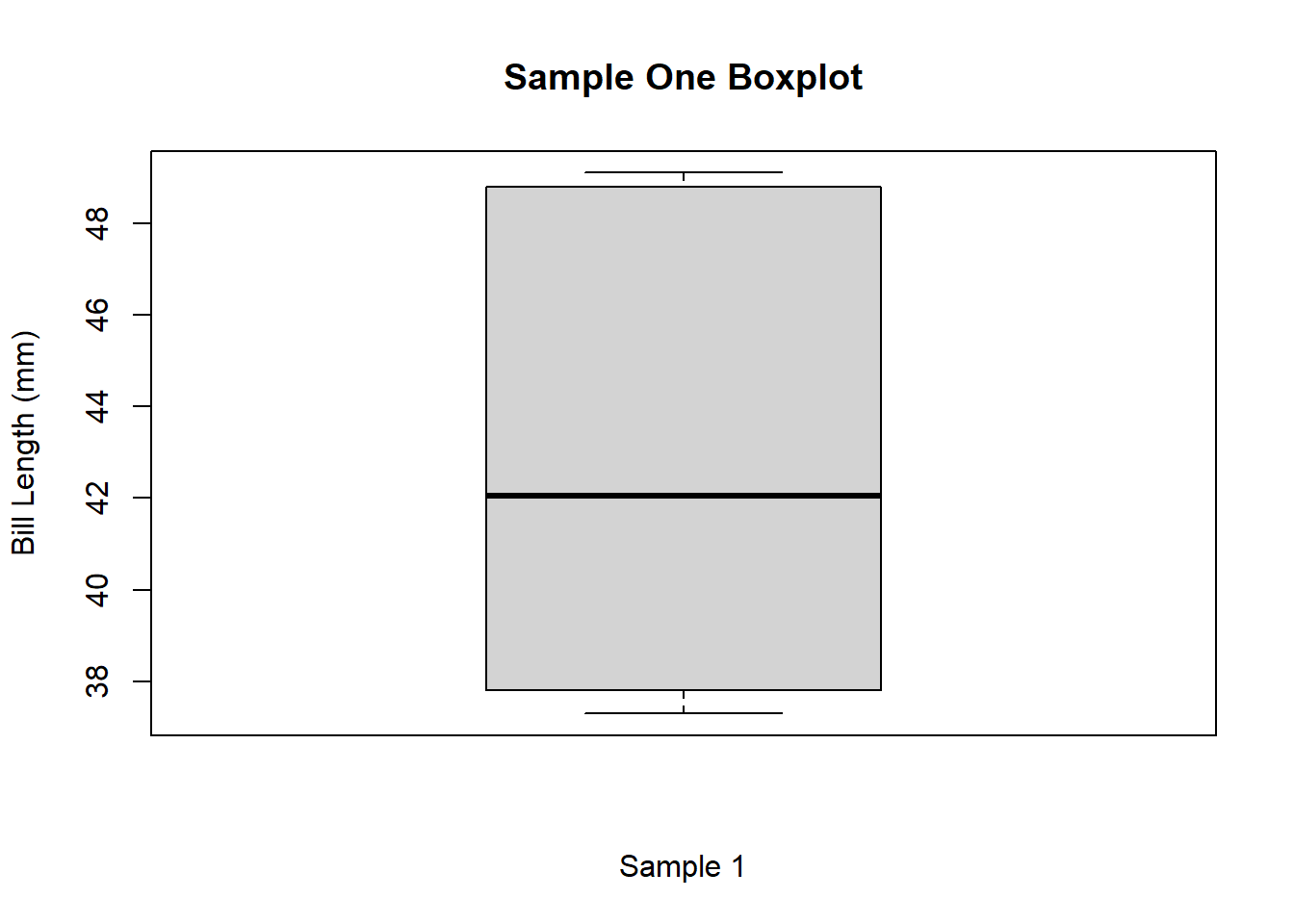
Example 11.11 (Boxplots and Numeric Summaries) Charles and Sadie have gotten very much into the summarizing data from the penguins. For the first sample of penguins, they have measurements of bill lengths in mm, with the following observations.

49.0

37.8

45.8

39.0

43.2

48.8

37.8

49.1

40.9

37.3

They took another two samples with other bill length measurements, but seemed to have lost the data directly. Fortunately, they have the five number summaries. These are given by the following.

Sample	Min	Q1	Median	Q3	Max
2	32	40	43	45	52
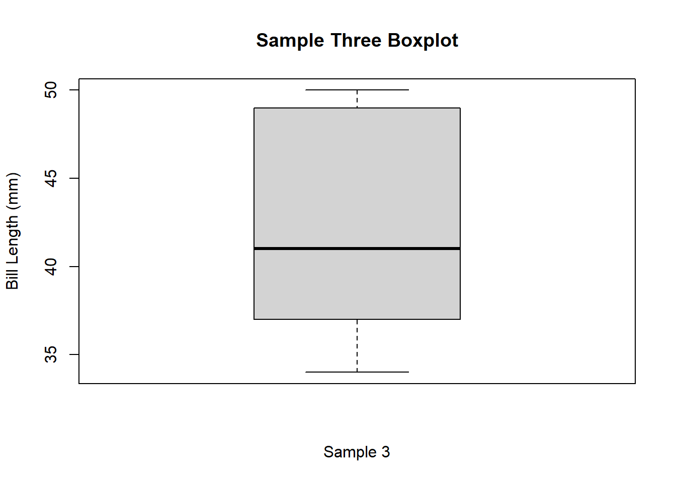
3	34	37	41	49	50

1. Write down the five number summary for the first sample.
2. Sketch a boxplot for the first sample, or explain why it is not possible.
3. Sketch a boxplot for the second sample, or explain why it is not possible.
4. Sketch a boxplot for the third sample, or explain why it is not possible.

Solution

1. In the previous examples, Example 11.8 and Example 11.10, we found that the five number summary would be given by \(37.3, 37.8, 42.05, 48.8, 49.1\).
2. The boxplot here will have a box drawn from \(37.8\) to \(48.8\), with a median line drawn at \(42.05\). The whiskers will extend for \(37.3\) which is only \(0.5\) beneath \(Q1\) and so there will be no outlier points drawn. The upper whisker will be drawn out to \(49.1\) which is only \(0.3\) above \(Q3\) and so it will be drawn without outlier points. This can be pictured as follows.

3. In this case we will be unable to draw a boxplot for the sample. The issue is that the minimum point is \(32\) which is \(8\) below \(Q1\). The IQR is \(45 - 40 = 5\), and so \(1.5\times 5 = 7.5\). As a result, the minimum would need to be drawn as an outlier point, which means that we cannot know where the whiskers will stop. This concern is not present on the upper side, where the whisker would be extended to \(52\).
4. Here we can use the \(5\) number summary to draw the boxplot directly. The box would be drawn from \(37\) to \(49\), with the medina marked at \(41\). The whiskers would extend down to \(34\) (\(3\) below \(Q1\)) and up to \(50\) (\(1\) above \(Q3\)). This can be pictured as follows.

It is important to note that the boxplot is inspired by the five number summary, but it encodes slightly more information. It will be precisely the same whenever the maximum and minimum fall within \(1.5\) times the IQR of the first and third quartiles, but it will include further information in all other cases. This is done to indicate points which are outliers, those which appear to deviate from expected trends (of nicely behaved data).¹⁵

Typically, the boxplots will be drawn so that multiple plots are shown on the same graph. In order to read a boxplot you can compare the medians, and then the spread. The typical variability of the quantity is contained within the box portion, and plots which have largely overlapping boxes are often thought to behave similarly. The whiskers represent the outer limits of what is expected within the data: if both whiskers are roughly the same length, the distribution appears to be mostly symmetric. If one is longer than the other, the distribution exhibits either positive or negative skew. The outliers can contribute to the illustration of skewness on the distribution, but are typically less representative of the distribution itself. A boxplot with a lot of outliers is suggestive of a dataset with far heavier tails than is typical for most well-behaved data, and any analysis on these data should proceed cautiously.

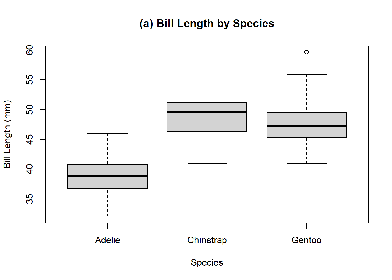
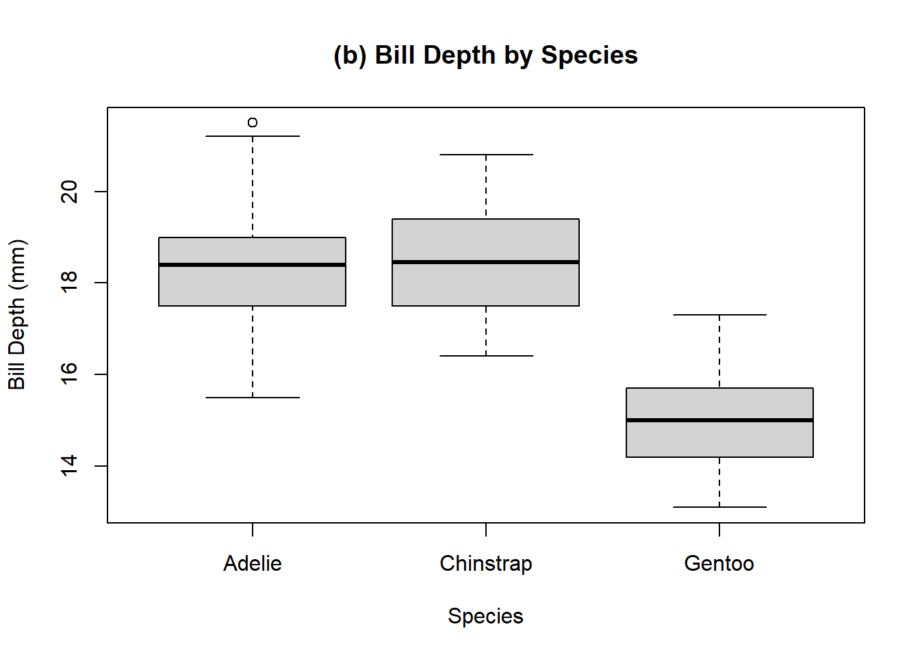
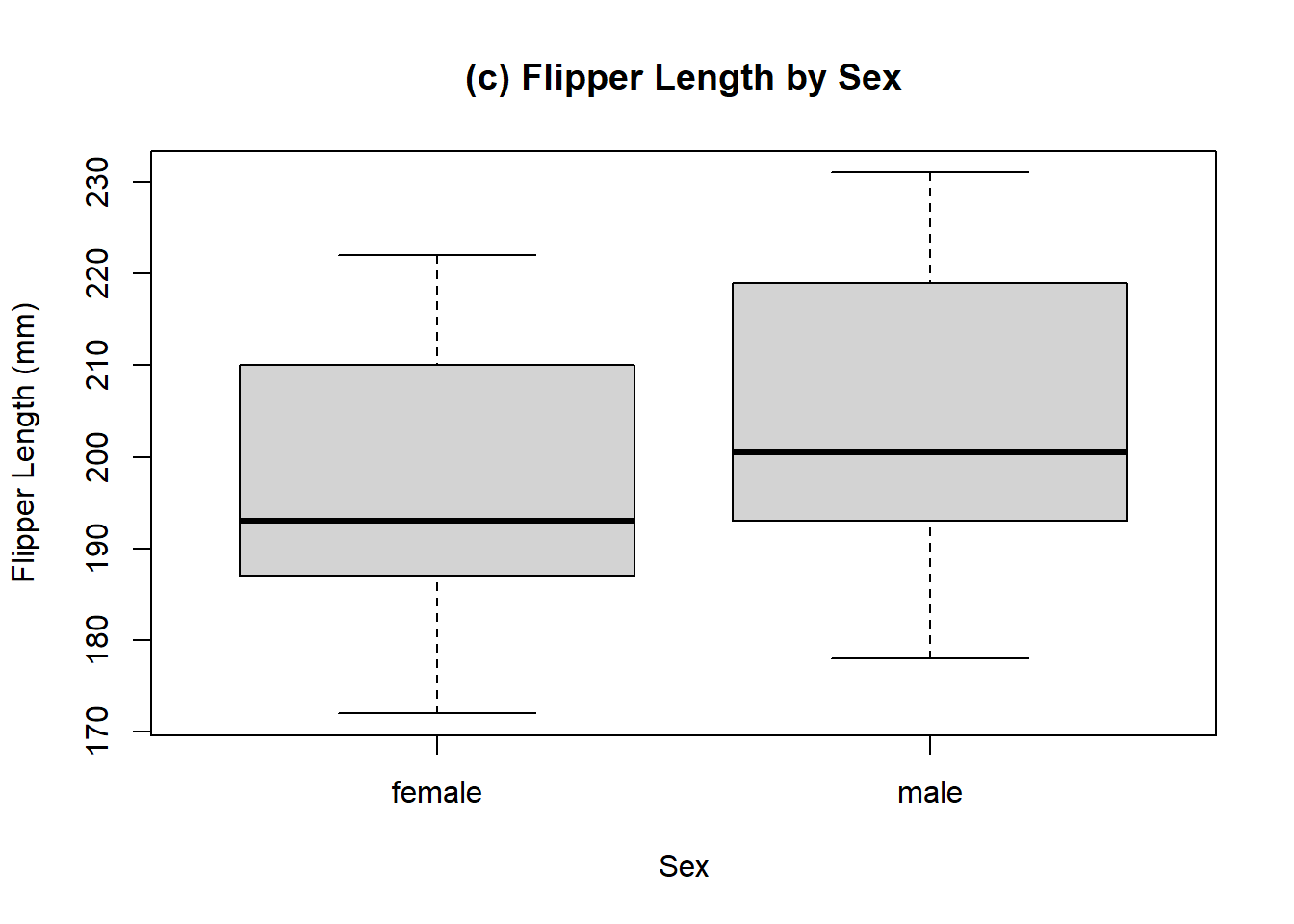
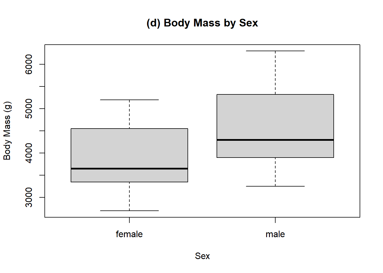
Example 11.12 (Penguin Species Comparisons) The enthusiasm that Charles and Sadie had for the penguin data lead them to reaching out to some researchers who have actually studied the penguins. The researchers, grateful to share their work with enthusiastic individuals, sent a series of boxplots comparing multiple different measurements broken up by penguing species and by the sex of the penguins. Charles and Sadie begin to study these various boxplots, comparing the distributions illustrated by each of the boxplots, and trying to determine differences in observations. For each of the following boxplots, compare the location and spread of the various distributions represented, and briefly describe what is observed. The following boxplots are given for:

1. Bill length by species.
2. Bill depth by species.
3. Flipper length by sex.
4. Body mass by sex.

Solution

1. By way of comparison, the adelie pegnuins appear to have less long bills than both the chinstrap and the gentoos, even when accounting for variability. We can see this since the median is substantially lower, and the box does not appear to overlap at all. The chinstrap and gentoo have more comparable bill length,s with the chinstrap being slightly larger in general, but with the gentoo having extreme observations that are the longest observed.

   The adelie have a median of just below \(40\), will an interquartile range from about \(37\) to around \(41\), and all observations falling between about \(32\) and \(46\). The chinstrap have a median length around \(50\), with an interquartile range from about \(46\) through \(51\), and a full data span between about \(41\) and \(58\). The gentoo have a median of around \(47\), with a fairly small IQR, spanning from around \(46\) to around \(50\). There are no negative outliers, all points falling above about \(41\), but the highest point extends to nearly \(60\), sitting beyond the outlier limit of around \(56\).

   The specific five number summary (not easily read directly from the boxplots are):

	Adelie	Chinstrap	Gentoo
Min	32.10	40.90	40.90
Q1	36.75	46.30	45.30
Median	38.80	49.55	47.30
Q3	40.75	51.15	49.55
Max	46.00	58.00	59.60

2. The adelie an chinstrap penguins exhibit roughly the same location, with the chinstrap exhibiting slightly more variability in terms of IQR and slightly less variability in terms of the overall range. The gentoo have less deep bills than either of the other species, with very little overlap between them at all.

   The adlie have a median depth of around \(18.5\), with an IQR ranging from just under \(18\) to around \(19\). There is one outlying observation, sitting above \(21\), with no outliers in the negative direction. The smallest observed bill depth is around \(15.5\). The chinstrap have a similar median, again around \(18.5\), with an IQR spanning from just below \(18\) to just over \(19\). The range of the data, however, sit from around \(16.5\) through to approxiamtely \(21\), with no extreme outlying observations. The gentoo have a median that is a little ways above \(15\), with an IQR from just above \(14\) to around \(16\). The range of the data in total is from around \(13\) to around \(17\).

   The specific five number summary (not easily read directly from the boxplots are):

	Adelie	Chinstrap	Gentoo
Min	15.5	16.40	13.1
Q1	17.5	17.50	14.2
Median	18.4	18.45	15.0
Q3	19.0	19.40	15.7
Max	21.5	20.80	17.3

3. Male penguins have slightly longer flippers, on average, but with fairly substantial overlap. Both males and females tend to exhibit similar spread, both in terms of the IQR and the range of the data, and the it quite a lot of overlap for both. For each species, the median sits closer to the first quartile than the third quartile, which suggests that there is likely some skewness in the positive direction, at least throughout the bulk of theo bservations.

   To summarize each distribution, you should be able to determine the approximate locations of each of the five numbers from the summary. There are no outliers for any of the measurements. The specific five number summary (not easily read with specificity from the boxplots are):

	Female	Male
Min	172	178.0
Q1	187	193.0
Median	193	200.5
Q3	210	219.0
Max	222	231.0

4. Male penguins weigh more on average than the females. The male penguins also seem to exhibit a wider spread, both in terms of the IQR and the overall range. There is a substantial amount of overlap between the main data, however, less so than for flipper length. Just as with flipper length, the median sits closer to the first quartile than the third, suggesting that there is a slight positive skew in the data.

To summarize each distribution, you should be able to determine the approximate locations of each of the five numbers from the summary. There are no outliers for any of the measurements. The specific five number summary (not easily read with specificity from the boxplots are):

	Female	Male
Min	2700	3250
Q1	3350	3900
Median	3650	4300
Q3	4550	5325
Max	5200	6300

Exercises

Exercise 11.1 In a survey conducted among students, they were asked about their favourite colors. The options were red, blue, green, yellow, and orange. Below are the responses from 10 students. Use these data to construct a frequency distribution.

Red, Blue, Green, Yellow, Orange, Blue, Red, Green, Green, Yellow

Exercise 11.2 A group of students was surveyed about their preferred leisure activities. The options included reading, playing sports, watching movies, listening to music, and playing video games. Below are the responses from 15 students. Construct the frequency distribution for these data.

Reading, Playing Sports, Watching Movies, Listening to Music, Playing Video Games, Reading, Playing Sports, Watching Movies, Watching Movies, Listening to Music, Playing Video Games, Reading, Reading, Playing Sports, Playing Sports

Exercise 11.3 In a class of 30 students, each student was asked to choose their favourite genre of music from rock, pop, hip-hop, jazz, and classical. Below are the responses for 10 of them.

Rock, Pop, Pop, Hip-Hop, Jazz, Classical, Rock, Pop, Pop, Hip-Hop

1. Use these responses to construct a frequency distribution for the data.
2. What proportion of the \(30\) students preferred rock?

Exercise 11.4 A survey was conducted to find out how many pets each household owns. Below are the responses from 20 households.

2, 1, 3, 0, 2, 1, 4, 2, 0, 1, 2, 3, 2, 1, 5, 2, 3, 1, 0, 2

1. What type of variable is this?
2. Write down the frequency distribution for these data. What bin width should you use?
3. Find the five number summary for these data.
4. What is the mode for this variable?

Exercise 11.5 The number of books read by students over the summer break was collected. Below are the responses from 8 students.

4, 6, 2, 1, 3, 0, 1, 3

1. Write down the frequency distribution for these data.
2. Find the five number summary for these data.
3. Find the mean and standard deviation for these data.

Exercise 11.6 The time taken (in minutes) by students to complete a quiz was recorded. Below are the times taken by 20 students.

20, 25, 30, 35, 40, 22, 28, 33, 37, 42, 24, 29, 31, 36, 39, 21, 26, 32, 38, 41

1. What type of variable is this best treated as?
2. Write down a frequency distribution for these data. What bin width did you use?
3. Find the five number summary for these data.
4. What is the mode for this variable?

Exercise 11.7 A survey asked participants about their monthly expenses on groceries, ranging from $100 to $1000. Below are the reported expenses from 5 participants.

251, 326, 182, 509, 427

1. Write down the frequency distribution for these data.
2. Find the five number summary for these data.
3. Find the mean and standard deviation for these data.

Exercise 11.8 Consider the following histogram displaying the distribution of volumes for black cherry trees.

1. Describe the distribution of the data set.
2. What is the bin width used?
3. What is the relative frequency of trees between \(10\) and \(20\) cubic feet?
4. Are there any notable outliers, (points which otherwise seem to deviate from the overall pattern)? Describe why this may be the case.
5. How would the relative frequency between \(10\) and \(20\) change if \(4\) observations between \(60\) and \(70\) were added?

Exercise 11.9 Consider the following histogram displaying the distribution of heights for black cherry trees.

1. Describe the distribution of the data set.
2. What is the bin width used?
3. What is the relative frequency of trees between \(70\) and \(75\) cubic feet?
4. Are there any notable outliers, (points which otherwise seem to deviate from the overall pattern)? Describe why this may be the case.

Exercise 11.10 Consider the following histogram displaying the distribution of lengths of major rivers in the US.

1. Describe the distribution of the data set.
2. What is the bin width used?
3. Are there any notable outliers, (points which otherwise seem to deviate from the overall pattern)? Describe why this may be the case.
4. When might this be an effective plot? When might this plot be ineffective?
5. Approximately what percentage of observations were longer than \(2000\)?

Exercise 11.11 Consider the following histogram displaying the distribution of lengths of major rivers in the US, containing only the data on the rivers under \(2000\) miles.

1. Describe the distribution of the data set.
2. How many bins are there?
3. Are there any notable outliers, (points which otherwise seem to deviate from the overall pattern)? Describe why this may be the case.
4. Describe how the previous histogram (from Exercise 11.10) would change if the bin width for this graph were used.
5. Approximately what percentage of observations fell between \(1000\) and \(1500\)?

Exercise 11.12 Consider the following histogram depicting industrial pressure measurements.

1. Describe the distribution of the data set.
2. What is the bin width used?
3. Are there any notable outliers, (points which otherwise seem to deviate from the overall pattern)? Describe why this may be the case.
4. Suppose that measurements beyond \(100\) are known to be the result of a transcription error, and they actually should have been recorded between \(90\) and \(95\). Describe the distribution that would arise.
5. Approximately what proportion of observations were below \(75\) or above \(90\)?

Exercise 11.13 Data from the file used to generate the following histogram was accidentally deleted where observations from the independent variable equaled \(4\). If there were \(240\) total observations, how many observations were for \(4\)?

Exercise 11.14 Consider the following histogram displaying the distribution of volumes for black cherry trees.

Using the plot, answer the following:

1. What is the median of the distribution?
2. What is the approximate mean of the distribution?
3. What is the mode of the distribution?
4. Which measure of central tendency is the best for the distribution?
5. Calculate (or approximate) several measures of variation for the distribution.

Exercise 11.15 Consider the following histogram displaying the distribution of heights for black cherry trees.

Using the plot, answer the following:

1. What is the median of the distribution?
2. What is the approximate mean of the distribution?
3. What is the mode of the distribution?
4. Which measure of central tendency is the best for the distribution?
5. Calculate (or approximate) several measures of variation for the distribution.

Exercise 11.16 Consider the following histogram displaying the distribution of lengths of major rivers in the US.

Using the plot, answer the following:

1. What is the median of the distribution?
2. What is the approximate mean of the distribution?
3. What is the mode of the distribution?
4. Which measure of central tendency is the best for the distribution?
5. Calculate (or approximate) several measures of variation for the distribution.

Exercise 11.17 Consider the following histogram displaying the distribution of lengths of major rivers in the US, containing only the data on the rivers under \(2000\) miles.

Using the plot, answer the following:

1. What is the median of the distribution?
2. What is the approximate mean of the distribution?
3. What is the mode of the distribution?
4. Which measure of central tendency is the best for the distribution?
5. Will the measure of variation be larger or smaller when you restrict to the shorter rivers?

Exercise 11.18 Consider the following histogram depicting industrial pressure measurements.

Using the plot, answer the following:

1. What is the median of the distribution?
2. What is the approximate mean of the distribution?
3. What is the mode of the distribution?
4. Which measure of central tendency is the best for the distribution?
5. Calculate (or approximate) several measures of variation for the distribution.
6. Suppose that measurements beyond \(100\) are known to be the result of a transcription error, and they actually should have been recorded between \(90\) and \(95\). What measure of central tendency is best for the distribution?

Exercise 11.19 Consider a quantitative variable measured in a dataset.

1. Is the sample mean always equal to one of the values in the sample? If. so, explain why. If not, give an example.
2. Is the sample median always equal to one of the values in the sample? If. so, explain why. If not, give an example.
3. Is the sample mode always equal to one of the values in the sample? If. so, explain why. If not, give an example.

Exercise 11.20 In one group of \(20\) individuals, the mean height was \(178\)cm. In a second group of \(30\) individuals the mean height was \(164\)cm. What is the mean height for both groups, when they are put together?

Exercise 11.21 There are \(10\) employees in a particular division of a company. Their salaries have a mean of \(70,000\), a median of \(55,000\), and a standard deviation of \(20,000\). The largest number on the list is \(100,000\).

A clerical error is made which enters the maximum value as a \(1,000,000\) rather than \(100,000\).

1. What is the mean of the altered data?
2. What is the median of the altered data?
3. What is the standard deviation of the altered data?

Exercise 11.22 Four research teams caught groups of ganges dolphins, consisting of \(15\), \(20\), \(10,\) and \(18\) dolphins each. The reported mean weights (in pounds) of the groups were \(162\), \(148\), \(153\) and \(140\), respectively. What was the overall mean of all the dolphins?

Exercise 11.23 A certain company is considering giving employees a weekly raise. Currently, the average weekly salary at the company is \(1000\), with a standard deviation of \(100\).

1. What would happen to the mean and standard deviation if a \(\$50\) raise were given to every employee?
2. What would happen to the mean and standard deviation if a \(5\%\) raise were given to every employee?

Exercise 11.24 Match each of the following boxplots (A)-(D), with the histograms (1)-(4).

Self-Assessment

Note: the following questions are still experimental. Please contact me if you have any issues with these components. This can be if there are incorrect answers, or if there are any technical concerns. Each question currently has an ID with it, randomized for each version. If you have issues, reporting the specific ID will allow for easier checking!

For each question, you can check your answer using the checkmark button. You can cycle through variants of the question by pressing the arrow icon.

Self Assessment 11.1

A group of students was asked for their favourite genre of music from rock, pop, hip-hop, jazz, and classical.

Below are 9 responses.

rock, hip-hop, classical, jazz, pop, rock, hip-hop, pop, jazz

Using these data, consider the following frequency distribution.

Option	Frequency	Relative Frequency
rock	(a)	(f)
pop	(b)	(g)
hip-hop	(c)	(h)
jazz	(d)	(i)
classical	(e)	(j)

Fill in each of the corresponding blanks.

(Question ID: 0559282069)

In a survey conducted among students, they were asked about their favourite colors. The options were red, blue, green, yellow, and orange.

Below are 14 responses.

blue, blue, green, yellow, blue, blue, red, green, yellow, blue, orange, yellow, yellow, orange

Using these data, consider the following frequency distribution.

Option	Frequency	Relative Frequency
red	(a)	(f)
blue	(b)	(g)
green	(c)	(h)
yellow	(d)	(i)
orange	(e)	(j)

Fill in each of the corresponding blanks.

(Question ID: 0251015970)

A group of students was asked for their favourite genre of music from rock, pop, hip-hop, jazz, and classical.

Below are 11 responses.

classical, jazz, classical, hip-hop, pop, hip-hop, classical, classical, rock, hip-hop, jazz

Using these data, consider the following frequency distribution.

Option	Frequency	Relative Frequency
rock	(a)	(f)
pop	(b)	(g)
hip-hop	(c)	(h)
jazz	(d)	(i)
classical	(e)	(j)

Fill in each of the corresponding blanks.

(Question ID: 0500339761)

A group of students was surveyed about their preferred leisure activities. The options included reading, playing sports, watching movies, listening to music, and playing video games.

Below are 9 responses.

watching movies, listening to music, listening to music, playing video games, reading, listening to music, watching movies, reading, watching movies

Using these data, consider the following frequency distribution.

Option	Frequency	Relative Frequency
reading	(a)	(f)
playing sports	(b)	(g)
watching movies	(c)	(h)
listening to music	(d)	(i)
playing video games	(e)	(j)

Fill in each of the corresponding blanks.

(Question ID: 0125550682)

The number of books read by students over the summer break was collected.

Below are 11 responses.

3, 1, 0, 1, 1, 0, 4+, 2, 1, 0, 3

Using these data, consider the following frequency distribution.

Option	Frequency	Relative Frequency
0	(a)	(f)
1	(b)	(g)
2	(c)	(h)
3	(d)	(i)
4+	(e)	(j)

Fill in each of the corresponding blanks.

(Question ID: 0432839712)

A survey was conducted to find out how many pets each household owns.

Below are 8 responses.

1, 4+, 1, 2, 1, 0, 3, 1

Using these data, consider the following frequency distribution.

Option	Frequency	Relative Frequency
0	(a)	(f)
1	(b)	(g)
2	(c)	(h)
3	(d)	(i)
4+	(e)	(j)

Fill in each of the corresponding blanks.

(Question ID: 0303001117)

A survey was conducted to find out how many pets each household owns.

Below are 14 responses.

1, 2, 1, 0, 3, 0, 3, 4+, 3, 2, 3, 1, 0, 3

Using these data, consider the following frequency distribution.

Option	Frequency	Relative Frequency
0	(a)	(f)
1	(b)	(g)
2	(c)	(h)
3	(d)	(i)
4+	(e)	(j)

Fill in each of the corresponding blanks.

(Question ID: 0927559843)

A group of students was asked for their favourite genre of music from rock, pop, hip-hop, jazz, and classical.

Below are 8 responses.

rock, pop, classical, hip-hop, rock, jazz, jazz, hip-hop

Using these data, consider the following frequency distribution.

Option	Frequency	Relative Frequency
rock	(a)	(f)
pop	(b)	(g)
hip-hop	(c)	(h)
jazz	(d)	(i)
classical	(e)	(j)

Fill in each of the corresponding blanks.

(Question ID: 0390300895)

The number of books read by students over the summer break was collected.

Below are 15 responses.

2, 2, 2, 4+, 0, 0, 2, 1, 3, 2, 3, 2, 1, 0, 3

Using these data, consider the following frequency distribution.

Option	Frequency	Relative Frequency
0	(a)	(f)
1	(b)	(g)
2	(c)	(h)
3	(d)	(i)
4+	(e)	(j)

Fill in each of the corresponding blanks.

(Question ID: 0956117316)

A group of students was asked for their favourite genre of music from rock, pop, hip-hop, jazz, and classical.

Below are 15 responses.

classical, hip-hop, rock, classical, jazz, jazz, classical, rock, hip-hop, rock, classical, rock, jazz, pop, hip-hop

Using these data, consider the following frequency distribution.

Option	Frequency	Relative Frequency
rock	(a)	(f)
pop	(b)	(g)
hip-hop	(c)	(h)
jazz	(d)	(i)
classical	(e)	(j)

Fill in each of the corresponding blanks.

(Question ID: 0385207410)

The number of books read by students over the summer break was collected.

Below are 8 responses.

2, 2, 3, 3, 1, 4+, 0, 3

Using these data, consider the following frequency distribution.

Option	Frequency	Relative Frequency
0	(a)	(f)
1	(b)	(g)
2	(c)	(h)
3	(d)	(i)
4+	(e)	(j)

Fill in each of the corresponding blanks.

(Question ID: 0996176265)

A group of students was asked for their favourite genre of music from rock, pop, hip-hop, jazz, and classical.

Below are 14 responses.

classical, hip-hop, pop, classical, pop, pop, classical, pop, rock, jazz, jazz, classical, pop, hip-hop

Using these data, consider the following frequency distribution.

Option	Frequency	Relative Frequency
rock	(a)	(f)
pop	(b)	(g)
hip-hop	(c)	(h)
jazz	(d)	(i)
classical	(e)	(j)

Fill in each of the corresponding blanks.

(Question ID: 0645902178)

In a survey conducted among students, they were asked about their favourite colors. The options were red, blue, green, yellow, and orange.

Below are 10 responses.

orange, red, red, red, yellow, red, blue, red, green, blue

Using these data, consider the following frequency distribution.

Option	Frequency	Relative Frequency
red	(a)	(f)
blue	(b)	(g)
green	(c)	(h)
yellow	(d)	(i)
orange	(e)	(j)

Fill in each of the corresponding blanks.

(Question ID: 0672350543)

A survey was conducted to find out how many pets each household owns.

Below are 14 responses.

4+, 2, 1, 1, 0, 3, 0, 0, 0, 3, 2, 3, 1, 2

Using these data, consider the following frequency distribution.

Option	Frequency	Relative Frequency
0	(a)	(f)
1	(b)	(g)
2	(c)	(h)
3	(d)	(i)
4+	(e)	(j)

Fill in each of the corresponding blanks.

(Question ID: 0800045695)

A group of students was asked for their favourite genre of music from rock, pop, hip-hop, jazz, and classical.

Below are 13 responses.

rock, jazz, pop, rock, classical, pop, classical, classical, classical, pop, jazz, rock, hip-hop

Using these data, consider the following frequency distribution.

Option	Frequency	Relative Frequency
rock	(a)	(f)
pop	(b)	(g)
hip-hop	(c)	(h)
jazz	(d)	(i)
classical	(e)	(j)

Fill in each of the corresponding blanks.

(Question ID: 0611708944)

A group of students was asked for their favourite genre of music from rock, pop, hip-hop, jazz, and classical.

Below are 12 responses.

classical, classical, jazz, pop, pop, hip-hop, pop, classical, hip-hop, jazz, classical, pop

Using these data, consider the following frequency distribution.

Option	Frequency	Relative Frequency
rock	(a)	(f)
pop	(b)	(g)
hip-hop	(c)	(h)
jazz	(d)	(i)
classical	(e)	(j)

Fill in each of the corresponding blanks.

(Question ID: 0415044518)

A survey was conducted to find out how many pets each household owns.

Below are 8 responses.

0, 0, 2, 0, 4+, 2, 4+, 4+

Using these data, consider the following frequency distribution.

Option	Frequency	Relative Frequency
0	(a)	(f)
1	(b)	(g)
2	(c)	(h)
3	(d)	(i)
4+	(e)	(j)

Fill in each of the corresponding blanks.

(Question ID: 0765029936)

A group of students was asked for their favourite genre of music from rock, pop, hip-hop, jazz, and classical.

Below are 15 responses.

classical, hip-hop, pop, rock, pop, classical, rock, pop, classical, hip-hop, classical, pop, classical, pop, classical

Using these data, consider the following frequency distribution.

Option	Frequency	Relative Frequency
rock	(a)	(f)
pop	(b)	(g)
hip-hop	(c)	(h)
jazz	(d)	(i)
classical	(e)	(j)

Fill in each of the corresponding blanks.

(Question ID: 0507752628)

In a survey conducted among students, they were asked about their favourite colors. The options were red, blue, green, yellow, and orange.

Below are 15 responses.

blue, blue, green, green, blue, yellow, yellow, blue, green, yellow, blue, green, yellow, red, orange

Using these data, consider the following frequency distribution.

Option	Frequency	Relative Frequency
red	(a)	(f)
blue	(b)	(g)
green	(c)	(h)
yellow	(d)	(i)
orange	(e)	(j)

Fill in each of the corresponding blanks.

(Question ID: 0609965474)

The number of books read by students over the summer break was collected.

Below are 15 responses.

0, 0, 4+, 0, 0, 2, 0, 0, 4+, 1, 4+, 3, 3, 0, 4+

Using these data, consider the following frequency distribution.

Option	Frequency	Relative Frequency
0	(a)	(f)
1	(b)	(g)
2	(c)	(h)
3	(d)	(i)
4+	(e)	(j)

Fill in each of the corresponding blanks.

(Question ID: 0059932786)

The number of books read by students over the summer break was collected.

Below are 13 responses.

2, 2, 0, 1, 1, 3, 4+, 0, 0, 0, 3, 1, 3

Using these data, consider the following frequency distribution.

Option	Frequency	Relative Frequency
0	(a)	(f)
1	(b)	(g)
2	(c)	(h)
3	(d)	(i)
4+	(e)	(j)

Fill in each of the corresponding blanks.

(Question ID: 0283863949)

The number of books read by students over the summer break was collected.

Below are 11 responses.

4+, 4+, 0, 1, 2, 3, 4+, 3, 3, 4+, 4+

Using these data, consider the following frequency distribution.

Option	Frequency	Relative Frequency
0	(a)	(f)
1	(b)	(g)
2	(c)	(h)
3	(d)	(i)
4+	(e)	(j)

Fill in each of the corresponding blanks.

(Question ID: 0376847247)

The number of books read by students over the summer break was collected.

Below are 8 responses.

4+, 3, 2, 2, 2, 1, 1, 0

Using these data, consider the following frequency distribution.

Option	Frequency	Relative Frequency
0	(a)	(f)
1	(b)	(g)
2	(c)	(h)
3	(d)	(i)
4+	(e)	(j)

Fill in each of the corresponding blanks.

(Question ID: 0599324713)

A survey was conducted to find out how many pets each household owns.

Below are 12 responses.

3, 1, 4+, 1, 4+, 4+, 3, 2, 1, 4+, 4+, 1

Using these data, consider the following frequency distribution.

Option	Frequency	Relative Frequency
0	(a)	(f)
1	(b)	(g)
2	(c)	(h)
3	(d)	(i)
4+	(e)	(j)

Fill in each of the corresponding blanks.

(Question ID: 0916017075)

A group of students was asked for their favourite genre of music from rock, pop, hip-hop, jazz, and classical.

Below are 8 responses.

rock, rock, rock, hip-hop, classical, rock, rock, jazz

Using these data, consider the following frequency distribution.

Option	Frequency	Relative Frequency
rock	(a)	(f)
pop	(b)	(g)
hip-hop	(c)	(h)
jazz	(d)	(i)
classical	(e)	(j)

Fill in each of the corresponding blanks.

(Question ID: 0571980000)

A group of students was asked for their favourite genre of music from rock, pop, hip-hop, jazz, and classical.

Below are 8 responses.

hip-hop, pop, hip-hop, jazz, rock, jazz, classical, hip-hop

Using these data, consider the following frequency distribution.

Option	Frequency	Relative Frequency
rock	(a)	(f)
pop	(b)	(g)
hip-hop	(c)	(h)
jazz	(d)	(i)
classical	(e)	(j)

Fill in each of the corresponding blanks.

(Question ID: 0462256162)

In a survey conducted among students, they were asked about their favourite colors. The options were red, blue, green, yellow, and orange.

Below are 14 responses.

yellow, green, orange, red, blue, blue, yellow, yellow, yellow, blue, green, yellow, blue, orange

Using these data, consider the following frequency distribution.

Option	Frequency	Relative Frequency
red	(a)	(f)
blue	(b)	(g)
green	(c)	(h)
yellow	(d)	(i)
orange	(e)	(j)

Fill in each of the corresponding blanks.

(Question ID: 0492462676)

A group of students was asked for their favourite genre of music from rock, pop, hip-hop, jazz, and classical.

Below are 8 responses.

jazz, pop, classical, rock, pop, rock, jazz, pop

Using these data, consider the following frequency distribution.

Option	Frequency	Relative Frequency
rock	(a)	(f)
pop	(b)	(g)
hip-hop	(c)	(h)
jazz	(d)	(i)
classical	(e)	(j)

Fill in each of the corresponding blanks.

(Question ID: 0914365443)

The number of books read by students over the summer break was collected.

Below are 13 responses.

4+, 3, 3, 1, 3, 2, 0, 4+, 4+, 4+, 3, 2, 4+

Using these data, consider the following frequency distribution.

Option	Frequency	Relative Frequency
0	(a)	(f)
1	(b)	(g)
2	(c)	(h)
3	(d)	(i)
4+	(e)	(j)

Fill in each of the corresponding blanks.

(Question ID: 0957176680)

The number of books read by students over the summer break was collected.

Below are 9 responses.

2, 0, 0, 4+, 4+, 1, 1, 2, 0

Using these data, consider the following frequency distribution.

Option	Frequency	Relative Frequency
0	(a)	(f)
1	(b)	(g)
2	(c)	(h)
3	(d)	(i)
4+	(e)	(j)

Fill in each of the corresponding blanks.

(Question ID: 0857224313)

A group of students was asked for their favourite genre of music from rock, pop, hip-hop, jazz, and classical.

Below are 14 responses.

rock, hip-hop, hip-hop, hip-hop, hip-hop, hip-hop, pop, jazz, pop, classical, hip-hop, pop, jazz, rock

Using these data, consider the following frequency distribution.

Option	Frequency	Relative Frequency
rock	(a)	(f)
pop	(b)	(g)
hip-hop	(c)	(h)
jazz	(d)	(i)
classical	(e)	(j)

Fill in each of the corresponding blanks.

(Question ID: 0605825385)

A group of students was asked for their favourite genre of music from rock, pop, hip-hop, jazz, and classical.

Below are 13 responses.

hip-hop, rock, hip-hop, rock, hip-hop, hip-hop, pop, pop, pop, hip-hop, jazz, rock, hip-hop

Using these data, consider the following frequency distribution.

Option	Frequency	Relative Frequency
rock	(a)	(f)
pop	(b)	(g)
hip-hop	(c)	(h)
jazz	(d)	(i)
classical	(e)	(j)

Fill in each of the corresponding blanks.

(Question ID: 0938548562)

In a survey conducted among students, they were asked about their favourite colors. The options were red, blue, green, yellow, and orange.

Below are 10 responses.

orange, green, yellow, blue, green, yellow, yellow, green, yellow, green

Using these data, consider the following frequency distribution.

Option	Frequency	Relative Frequency
red	(a)	(f)
blue	(b)	(g)
green	(c)	(h)
yellow	(d)	(i)
orange	(e)	(j)

Fill in each of the corresponding blanks.

(Question ID: 0032500961)

The number of books read by students over the summer break was collected.

Below are 11 responses.

3, 4+, 4+, 0, 1, 4+, 3, 0, 2, 3, 3

Using these data, consider the following frequency distribution.

Option	Frequency	Relative Frequency
0	(a)	(f)
1	(b)	(g)
2	(c)	(h)
3	(d)	(i)
4+	(e)	(j)

Fill in each of the corresponding blanks.

(Question ID: 0013327127)

The number of books read by students over the summer break was collected.

Below are 15 responses.

1, 1, 2, 1, 1, 2, 3, 3, 3, 3, 3, 0, 1, 0, 3

Using these data, consider the following frequency distribution.

Option	Frequency	Relative Frequency
0	(a)	(f)
1	(b)	(g)
2	(c)	(h)
3	(d)	(i)
4+	(e)	(j)

Fill in each of the corresponding blanks.

(Question ID: 0135393923)

A group of students was asked for their favourite genre of music from rock, pop, hip-hop, jazz, and classical.

Below are 8 responses.

pop, hip-hop, jazz, classical, hip-hop, pop, classical, pop

Using these data, consider the following frequency distribution.

Option	Frequency	Relative Frequency
rock	(a)	(f)
pop	(b)	(g)
hip-hop	(c)	(h)
jazz	(d)	(i)
classical	(e)	(j)

Fill in each of the corresponding blanks.

(Question ID: 0806820397)

A survey was conducted to find out how many pets each household owns.

Below are 9 responses.

1, 1, 2, 1, 4+, 2, 3, 4+, 4+

Using these data, consider the following frequency distribution.

Option	Frequency	Relative Frequency
0	(a)	(f)
1	(b)	(g)
2	(c)	(h)
3	(d)	(i)
4+	(e)	(j)

Fill in each of the corresponding blanks.

(Question ID: 0074817175)

In a survey conducted among students, they were asked about their favourite colors. The options were red, blue, green, yellow, and orange.

Below are 10 responses.

red, green, yellow, red, green, red, orange, red, yellow, yellow

Using these data, consider the following frequency distribution.

Option	Frequency	Relative Frequency
red	(a)	(f)
blue	(b)	(g)
green	(c)	(h)
yellow	(d)	(i)
orange	(e)	(j)

Fill in each of the corresponding blanks.

(Question ID: 0479416509)

The number of books read by students over the summer break was collected.

Below are 15 responses.

3, 1, 0, 4+, 0, 1, 3, 3, 4+, 1, 3, 4+, 2, 2, 2

Using these data, consider the following frequency distribution.

Option	Frequency	Relative Frequency
0	(a)	(f)
1	(b)	(g)
2	(c)	(h)
3	(d)	(i)
4+	(e)	(j)

Fill in each of the corresponding blanks.

(Question ID: 0426861956)

In a survey conducted among students, they were asked about their favourite colors. The options were red, blue, green, yellow, and orange.

Below are 14 responses.

yellow, blue, yellow, orange, green, yellow, orange, blue, green, orange, red, blue, green, green

Using these data, consider the following frequency distribution.

Option	Frequency	Relative Frequency
red	(a)	(f)
blue	(b)	(g)
green	(c)	(h)
yellow	(d)	(i)
orange	(e)	(j)

Fill in each of the corresponding blanks.

(Question ID: 0212195253)

A group of students was asked for their favourite genre of music from rock, pop, hip-hop, jazz, and classical.

Below are 13 responses.

rock, rock, pop, hip-hop, jazz, jazz, hip-hop, jazz, pop, hip-hop, pop, classical, jazz

Using these data, consider the following frequency distribution.

Option	Frequency	Relative Frequency
rock	(a)	(f)
pop	(b)	(g)
hip-hop	(c)	(h)
jazz	(d)	(i)
classical	(e)	(j)

Fill in each of the corresponding blanks.

(Question ID: 0562290162)

In a survey conducted among students, they were asked about their favourite colors. The options were red, blue, green, yellow, and orange.

Below are 8 responses.

yellow, yellow, green, red, yellow, red, blue, red

Using these data, consider the following frequency distribution.

Option	Frequency	Relative Frequency
red	(a)	(f)
blue	(b)	(g)
green	(c)	(h)
yellow	(d)	(i)
orange	(e)	(j)

Fill in each of the corresponding blanks.

(Question ID: 0792206038)

In a survey conducted among students, they were asked about their favourite colors. The options were red, blue, green, yellow, and orange.

Below are 10 responses.

blue, green, orange, green, yellow, blue, red, yellow, red, yellow

Using these data, consider the following frequency distribution.

Option	Frequency	Relative Frequency
red	(a)	(f)
blue	(b)	(g)
green	(c)	(h)
yellow	(d)	(i)
orange	(e)	(j)

Fill in each of the corresponding blanks.

(Question ID: 0038517045)

A group of students was surveyed about their preferred leisure activities. The options included reading, playing sports, watching movies, listening to music, and playing video games.

Below are 8 responses.

playing sports, playing sports, reading, listening to music, playing sports, listening to music, reading, playing sports

Using these data, consider the following frequency distribution.

Option	Frequency	Relative Frequency
reading	(a)	(f)
playing sports	(b)	(g)
watching movies	(c)	(h)
listening to music	(d)	(i)
playing video games	(e)	(j)

Fill in each of the corresponding blanks.

(Question ID: 0250708588)

In a survey conducted among students, they were asked about their favourite colors. The options were red, blue, green, yellow, and orange.

Below are 11 responses.

yellow, blue, blue, green, blue, green, red, red, red, blue, orange

Using these data, consider the following frequency distribution.

Option	Frequency	Relative Frequency
red	(a)	(f)
blue	(b)	(g)
green	(c)	(h)
yellow	(d)	(i)
orange	(e)	(j)

Fill in each of the corresponding blanks.

(Question ID: 0910045891)

The number of books read by students over the summer break was collected.

Below are 13 responses.

0, 3, 1, 4+, 0, 1, 0, 2, 1, 2, 2, 3, 0

Using these data, consider the following frequency distribution.

Option	Frequency	Relative Frequency
0	(a)	(f)
1	(b)	(g)
2	(c)	(h)
3	(d)	(i)
4+	(e)	(j)

Fill in each of the corresponding blanks.

(Question ID: 0056713185)

A group of students was surveyed about their preferred leisure activities. The options included reading, playing sports, watching movies, listening to music, and playing video games.

Below are 9 responses.

reading, playing video games, listening to music, listening to music, listening to music, reading, playing video games, playing sports, playing video games

Using these data, consider the following frequency distribution.

Option	Frequency	Relative Frequency
reading	(a)	(f)
playing sports	(b)	(g)
watching movies	(c)	(h)
listening to music	(d)	(i)
playing video games	(e)	(j)

Fill in each of the corresponding blanks.

(Question ID: 0688122892)

In a survey conducted among students, they were asked about their favourite colors. The options were red, blue, green, yellow, and orange.

Below are 10 responses.

yellow, red, yellow, orange, yellow, blue, yellow, orange, green, yellow

Using these data, consider the following frequency distribution.

Option	Frequency	Relative Frequency
red	(a)	(f)
blue	(b)	(g)
green	(c)	(h)
yellow	(d)	(i)
orange	(e)	(j)

Fill in each of the corresponding blanks.

(Question ID: 0870521544)

The number of books read by students over the summer break was collected.

Below are 15 responses.

3, 0, 3, 4+, 2, 2, 1, 1, 3, 0, 1, 4+, 4+, 4+, 1

Using these data, consider the following frequency distribution.

Option	Frequency	Relative Frequency
0	(a)	(f)
1	(b)	(g)
2	(c)	(h)
3	(d)	(i)
4+	(e)	(j)

Fill in each of the corresponding blanks.

(Question ID: 0640213893)

A group of students was asked for their favourite genre of music from rock, pop, hip-hop, jazz, and classical.

Below are 8 responses.

hip-hop, hip-hop, pop, hip-hop, rock, classical, rock, rock

Using these data, consider the following frequency distribution.

Option	Frequency	Relative Frequency
rock	(a)	(f)
pop	(b)	(g)
hip-hop	(c)	(h)
jazz	(d)	(i)
classical	(e)	(j)

Fill in each of the corresponding blanks.

(Question ID: 0119867126)

Self Assessment 11.2

The time taken (in minutes) by students to complete a quiz was recorded.

Possible responses range from 15 to 90. Below are 12 responses, ordered from smallest to largest.

18, 18, 26, 26, 37, 50, 53, 64, 71, 72, 73, 73

Suppose that there is a desire to have 3 bins in the frequency distribution.

1. What is the corresponding bin width?
2. What is the maximum value of the first bin?
3. What is the frequency of the largest bin?
4. What is the relative frequency of the 1st bin?

(Question ID: 0788958696)

The time taken (in minutes) by students to complete a quiz was recorded.

Possible responses range from 15 to 90. Below are 13 responses, ordered from smallest to largest.

17, 18, 22, 24, 29, 35, 40, 47, 55, 63, 66, 86, 90

Suppose that there is a desire to have 5 bins in the frequency distribution.

1. What is the corresponding bin width?
2. What is the maximum value of the first bin?
3. What is the frequency of the largest bin?
4. What is the relative frequency of the 1st bin?

(Question ID: 0590630894)

A survey asked homeowners about the age of their primary residence (in years).

Possible responses range from 0 to 150. Below are 11 responses, ordered from smallest to largest.

2, 35, 38, 39, 52, 53, 53, 99, 101, 111, 125

Suppose that there is a desire to have 2 bins in the frequency distribution.

1. What is the corresponding bin width?
2. What is the maximum value of the first bin?
3. What is the frequency of the largest bin?
4. What is the relative frequency of the 2nd bin?

(Question ID: 0189126905)

The blood pressure (systolic) of patients was measured during a routine check-up (in mmHg).

Possible responses range from 90 to 180. Below are 9 responses, ordered from smallest to largest.

103, 106, 107, 108, 115, 146, 157, 160, 164

Suppose that there is a desire to have 5 bins in the frequency distribution.

1. What is the corresponding bin width?
2. What is the maximum value of the first bin?
3. What is the frequency of the largest bin?
4. What is the relative frequency of the 4th bin?

(Question ID: 0458510174)

Participants were asked to estimate the number of hours they spend exercising per week.

Possible responses range from 0 to 40. Below are 11 responses, ordered from smallest to largest.

7, 13, 14, 16, 21, 28, 30, 32, 33, 35, 36

Suppose that there is a desire to have 10 bins in the frequency distribution.

1. What is the corresponding bin width?
2. What is the maximum value of the first bin?
3. What is the frequency of the largest bin?
4. What is the relative frequency of the 10th bin?

(Question ID: 0351699849)

A soil sample was analyzed for its pH level.

Possible responses range from 3.5 to 8.5. Below are 13 responses, ordered from smallest to largest.

3.97, 4.62, 5.11, 5.28, 5.5, 5.6, 5.77, 6.71, 6.75, 7.03, 7.15, 7.89, 8.45

Suppose that there is a desire to have 2 bins in the frequency distribution.

1. What is the corresponding bin width?
2. What is the maximum value of the first bin?
3. What is the frequency of the largest bin?
4. What is the relative frequency of the 2nd bin?

(Question ID: 0385254351)

The blood pressure (systolic) of patients was measured during a routine check-up (in mmHg).

Possible responses range from 90 to 180. Below are 11 responses, ordered from smallest to largest.

92, 104, 109, 134, 134, 143, 145, 149, 151, 158, 161

Suppose that there is a desire to have 3 bins in the frequency distribution.

1. What is the corresponding bin width?
2. What is the maximum value of the first bin?
3. What is the frequency of the largest bin?
4. What is the relative frequency of the 2nd bin?

(Question ID: 0967095252)

The concentration of a chemical pollutant in a water sample was measured (in parts per million).

Possible responses range from 0 to 5. Below are 11 responses, ordered from smallest to largest.

0.35, 0.36, 0.73, 1.03, 1.44, 1.48, 2.33, 2.45, 2.59, 2.98, 3.66

Suppose that there is a desire to have 2 bins in the frequency distribution.

1. What is the corresponding bin width?
2. What is the maximum value of the first bin?
3. What is the frequency of the largest bin?
4. What is the relative frequency of the 1st bin?

(Question ID: 0586656658)

The time taken (in minutes) by students to complete a quiz was recorded.

Possible responses range from 15 to 90. Below are 10 responses, ordered from smallest to largest.

38, 41, 52, 57, 59, 62, 71, 72, 77, 77

Suppose that there is a desire to have 5 bins in the frequency distribution.

1. What is the corresponding bin width?
2. What is the maximum value of the first bin?
3. What is the frequency of the largest bin?
4. What is the relative frequency of the 5th bin?

(Question ID: 0049371959)

Participants were asked to estimate the number of hours they spend exercising per week.

Possible responses range from 0 to 40. Below are 15 responses, ordered from smallest to largest.

7, 13, 17, 23, 24, 25, 27, 27, 30, 32, 36, 36, 37, 37, 38

Suppose that there is a desire to have 2 bins in the frequency distribution.

1. What is the corresponding bin width?
2. What is the maximum value of the first bin?
3. What is the frequency of the largest bin?
4. What is the relative frequency of the 2nd bin?

(Question ID: 0321980101)

The blood pressure (systolic) of patients was measured during a routine check-up (in mmHg).

Possible responses range from 90 to 180. Below are 10 responses, ordered from smallest to largest.

90, 91, 99, 106, 112, 141, 142, 159, 161, 170

Suppose that there is a desire to have 6 bins in the frequency distribution.

1. What is the corresponding bin width?
2. What is the maximum value of the first bin?
3. What is the frequency of the largest bin?
4. What is the relative frequency of the 3rd bin?

(Question ID: 0011900299)

A survey asked homeowners about the age of their primary residence (in years).

Possible responses range from 0 to 150. Below are 13 responses, ordered from smallest to largest.

7, 13, 38, 38, 39, 44, 47, 50, 51, 88, 108, 117, 140

Suppose that there is a desire to have 10 bins in the frequency distribution.

1. What is the corresponding bin width?
2. What is the maximum value of the first bin?
3. What is the frequency of the largest bin?
4. What is the relative frequency of the 5th bin?

(Question ID: 0298692892)

The height of adult males in a population was recorded (in centimeters).

Possible responses range from 150 to 210. Below are 11 responses, ordered from smallest to largest.

151, 157, 164, 166, 167, 176, 180, 182, 190, 205, 205

Suppose that there is a desire to have 2 bins in the frequency distribution.

1. What is the corresponding bin width?
2. What is the maximum value of the first bin?
3. What is the frequency of the largest bin?
4. What is the relative frequency of the 1st bin?

(Question ID: 0009068829)

The temperature (in degrees Celsius) of a liquid was measured using a digital thermometer.

Possible responses range from 0 to 95. Below are 13 responses, ordered from smallest to largest.

3.2, 8.69, 25.63, 32.18, 32.39, 34.95, 39.6, 53.77, 56.53, 59.49, 65.45, 83.04, 91.04

Suppose that there is a desire to have 2 bins in the frequency distribution.

1. What is the corresponding bin width?
2. What is the maximum value of the first bin?
3. What is the frequency of the largest bin?
4. What is the relative frequency of the 2nd bin?

(Question ID: 0176022555)

The blood pressure (systolic) of patients was measured during a routine check-up (in mmHg).

Possible responses range from 90 to 180. Below are 10 responses, ordered from smallest to largest.

94, 104, 108, 114, 148, 155, 164, 165, 166, 177

Suppose that there is a desire to have 3 bins in the frequency distribution.

1. What is the corresponding bin width?
2. What is the maximum value of the first bin?
3. What is the frequency of the largest bin?
4. What is the relative frequency of the 2nd bin?

(Question ID: 0869227082)

The concentration of a chemical pollutant in a water sample was measured (in parts per million).

Possible responses range from 0 to 5. Below are 10 responses, ordered from smallest to largest.

0.76, 1.11, 1.18, 1.68, 2.61, 2.83, 2.86, 3.05, 3.75, 4.42

Suppose that there is a desire to have 2 bins in the frequency distribution.

1. What is the corresponding bin width?
2. What is the maximum value of the first bin?
3. What is the frequency of the largest bin?
4. What is the relative frequency of the 1st bin?

(Question ID: 0951700812)

The response time (in milliseconds) of a website was recorded during a user testing session.

Possible responses range from 100 to 2000. Below are 14 responses, ordered from smallest to largest.

121, 213, 223, 264, 269, 284, 410, 506, 741, 769, 894, 1021, 1028, 1638

Suppose that there is a desire to have 5 bins in the frequency distribution.

1. What is the corresponding bin width?
2. What is the maximum value of the first bin?
3. What is the frequency of the largest bin?
4. What is the relative frequency of the 5th bin?

(Question ID: 0185212892)

The height of adult males in a population was recorded (in centimeters).

Possible responses range from 150 to 210. Below are 11 responses, ordered from smallest to largest.

152, 153, 166, 179, 182, 183, 184, 193, 193, 199, 207

Suppose that there is a desire to have 5 bins in the frequency distribution.

1. What is the corresponding bin width?
2. What is the maximum value of the first bin?
3. What is the frequency of the largest bin?
4. What is the relative frequency of the 1st bin?

(Question ID: 0559707919)

The concentration of a chemical pollutant in a water sample was measured (in parts per million).

Possible responses range from 0 to 5. Below are 13 responses, ordered from smallest to largest.

0.29, 0.45, 0.83, 0.94, 1.11, 1.6, 1.84, 3.07, 3.26, 3.96, 4, 4.08, 4.29

Suppose that there is a desire to have 2 bins in the frequency distribution.

1. What is the corresponding bin width?
2. What is the maximum value of the first bin?
3. What is the frequency of the largest bin?
4. What is the relative frequency of the 2nd bin?

(Question ID: 0778392389)

The temperature (in degrees Celsius) of a liquid was measured using a digital thermometer.

Possible responses range from 0 to 95. Below are 15 responses, ordered from smallest to largest.

5.37, 9, 14.58, 24.53, 25.32, 27.05, 36.51, 37.61, 49.77, 65.8, 76.31, 81.62, 83.19, 84.2, 88.85

Suppose that there is a desire to have 10 bins in the frequency distribution.

1. What is the corresponding bin width?
2. What is the maximum value of the first bin?
3. What is the frequency of the largest bin?
4. What is the relative frequency of the 1st bin?

(Question ID: 0457655792)

The height of adult males in a population was recorded (in centimeters).

Possible responses range from 150 to 210. Below are 10 responses, ordered from smallest to largest.

151, 153, 159, 161, 169, 188, 190, 194, 199, 208

Suppose that there is a desire to have 5 bins in the frequency distribution.

1. What is the corresponding bin width?
2. What is the maximum value of the first bin?
3. What is the frequency of the largest bin?
4. What is the relative frequency of the 2nd bin?

(Question ID: 0483804098)

The response time (in milliseconds) of a website was recorded during a user testing session.

Possible responses range from 100 to 2000. Below are 9 responses, ordered from smallest to largest.

689, 792, 906, 965, 1553, 1609, 1829, 1855, 1887

Suppose that there is a desire to have 2 bins in the frequency distribution.

1. What is the corresponding bin width?
2. What is the maximum value of the first bin?
3. What is the frequency of the largest bin?
4. What is the relative frequency of the 1st bin?

(Question ID: 0635141237)

The birthweights of infants at a neonatal ICU were recorded over the period of a month (in grams).

Possible responses range from 2000 to 5000. Below are 10 responses, ordered from smallest to largest.

2515, 2614, 3748, 3776, 3791, 3864, 4268, 4485, 4666, 4878

Suppose that there is a desire to have 8 bins in the frequency distribution.

1. What is the corresponding bin width?
2. What is the maximum value of the first bin?
3. What is the frequency of the largest bin?
4. What is the relative frequency of the 3rd bin?

(Question ID: 0441493429)

The response time (in milliseconds) of a website was recorded during a user testing session.

Possible responses range from 100 to 2000. Below are 14 responses, ordered from smallest to largest.

121, 173, 217, 251, 297, 406, 969, 1143, 1167, 1212, 1702, 1703, 1832, 1975

Suppose that there is a desire to have 10 bins in the frequency distribution.

1. What is the corresponding bin width?
2. What is the maximum value of the first bin?
3. What is the frequency of the largest bin?
4. What is the relative frequency of the 7th bin?

(Question ID: 0810132571)

A survey asked participants about their monthly expenses on groceries.

Possible responses range from 100 to 1000. Below are 11 responses, ordered from smallest to largest.

281, 368, 395, 566, 569, 617, 625, 632, 683, 821, 845

Suppose that there is a desire to have 9 bins in the frequency distribution.

1. What is the corresponding bin width?
2. What is the maximum value of the first bin?
3. What is the frequency of the largest bin?
4. What is the relative frequency of the 7th bin?

(Question ID: 0914173691)

The blood pressure (systolic) of patients was measured during a routine check-up (in mmHg).

Possible responses range from 90 to 180. Below are 15 responses, ordered from smallest to largest.

99, 102, 105, 115, 119, 131, 131, 140, 141, 149, 163, 164, 173, 176, 178

Suppose that there is a desire to have 3 bins in the frequency distribution.

1. What is the corresponding bin width?
2. What is the maximum value of the first bin?
3. What is the frequency of the largest bin?
4. What is the relative frequency of the 3rd bin?

(Question ID: 0211642247)

The temperature (in degrees Celsius) of a liquid was measured using a digital thermometer.

Possible responses range from 0 to 95. Below are 14 responses, ordered from smallest to largest.

20.28, 29, 43.9, 54.6, 55.49, 61.64, 71.96, 73.3, 76.56, 83.06, 83.12, 85.04, 90.62, 93.3

Suppose that there is a desire to have 10 bins in the frequency distribution.

1. What is the corresponding bin width?
2. What is the maximum value of the first bin?
3. What is the frequency of the largest bin?
4. What is the relative frequency of the 4th bin?

(Question ID: 0106989742)

The birthweights of infants at a neonatal ICU were recorded over the period of a month (in grams).

Possible responses range from 2000 to 5000. Below are 13 responses, ordered from smallest to largest.

2560, 2682, 3039, 3406, 3781, 4104, 4149, 4420, 4457, 4557, 4710, 4722, 4772

Suppose that there is a desire to have 5 bins in the frequency distribution.

1. What is the corresponding bin width?
2. What is the maximum value of the first bin?
3. What is the frequency of the largest bin?
4. What is the relative frequency of the 3rd bin?

(Question ID: 0676748067)

The blood pressure (systolic) of patients was measured during a routine check-up (in mmHg).

Possible responses range from 90 to 180. Below are 15 responses, ordered from smallest to largest.

96, 98, 99, 101, 107, 107, 111, 121, 124, 134, 140, 144, 146, 154, 172

Suppose that there is a desire to have 10 bins in the frequency distribution.

1. What is the corresponding bin width?
2. What is the maximum value of the first bin?
3. What is the frequency of the largest bin?
4. What is the relative frequency of the 5th bin?

(Question ID: 0408255707)

The height of adult males in a population was recorded (in centimeters).

Possible responses range from 150 to 210. Below are 14 responses, ordered from smallest to largest.

154, 156, 156, 180, 183, 183, 187, 187, 196, 200, 203, 206, 208, 208

Suppose that there is a desire to have 2 bins in the frequency distribution.

1. What is the corresponding bin width?
2. What is the maximum value of the first bin?
3. What is the frequency of the largest bin?
4. What is the relative frequency of the 2nd bin?

(Question ID: 0127234045)

The blood pressure (systolic) of patients was measured during a routine check-up (in mmHg).

Possible responses range from 90 to 180. Below are 15 responses, ordered from smallest to largest.

101, 106, 110, 111, 111, 113, 114, 120, 128, 138, 149, 160, 167, 171, 174

Suppose that there is a desire to have 3 bins in the frequency distribution.

1. What is the corresponding bin width?
2. What is the maximum value of the first bin?
3. What is the frequency of the largest bin?
4. What is the relative frequency of the 2nd bin?

(Question ID: 0309440581)

Participants were asked to estimate the number of hours they spend exercising per week.

Possible responses range from 0 to 40. Below are 13 responses, ordered from smallest to largest.

1, 11, 12, 15, 15, 15, 16, 21, 23, 25, 30, 38, 40

Suppose that there is a desire to have 4 bins in the frequency distribution.

1. What is the corresponding bin width?
2. What is the maximum value of the first bin?
3. What is the frequency of the largest bin?
4. What is the relative frequency of the 1st bin?

(Question ID: 0404035938)

Participants were asked to estimate the number of hours they spend exercising per week.

Possible responses range from 0 to 40. Below are 15 responses, ordered from smallest to largest.

2, 3, 5, 6, 9, 16, 21, 21, 22, 22, 32, 33, 34, 35, 38

Suppose that there is a desire to have 10 bins in the frequency distribution.

1. What is the corresponding bin width?
2. What is the maximum value of the first bin?
3. What is the frequency of the largest bin?
4. What is the relative frequency of the 2nd bin?

(Question ID: 0829889272)

The birthweights of infants at a neonatal ICU were recorded over the period of a month (in grams).

Possible responses range from 2000 to 5000. Below are 10 responses, ordered from smallest to largest.

2514, 2532, 2786, 3100, 3911, 3928, 4214, 4216, 4426, 4707

Suppose that there is a desire to have 3 bins in the frequency distribution.

1. What is the corresponding bin width?
2. What is the maximum value of the first bin?
3. What is the frequency of the largest bin?
4. What is the relative frequency of the 1st bin?

(Question ID: 0824488576)

The response time (in milliseconds) of a website was recorded during a user testing session.

Possible responses range from 100 to 2000. Below are 10 responses, ordered from smallest to largest.

260, 438, 775, 871, 1097, 1490, 1761, 1792, 1980, 1986

Suppose that there is a desire to have 5 bins in the frequency distribution.

1. What is the corresponding bin width?
2. What is the maximum value of the first bin?
3. What is the frequency of the largest bin?
4. What is the relative frequency of the 3rd bin?

(Question ID: 0780348937)

A survey asked homeowners about the age of their primary residence (in years).

Possible responses range from 0 to 150. Below are 14 responses, ordered from smallest to largest.

17, 21, 29, 31, 39, 41, 49, 50, 62, 63, 81, 87, 97, 117

Suppose that there is a desire to have 6 bins in the frequency distribution.

1. What is the corresponding bin width?
2. What is the maximum value of the first bin?
3. What is the frequency of the largest bin?
4. What is the relative frequency of the 4th bin?

(Question ID: 0581693828)

The time taken (in minutes) by students to complete a quiz was recorded.

Possible responses range from 15 to 90. Below are 12 responses, ordered from smallest to largest.

19, 24, 31, 35, 43, 48, 57, 60, 61, 64, 64, 85

Suppose that there is a desire to have 5 bins in the frequency distribution.

1. What is the corresponding bin width?
2. What is the maximum value of the first bin?
3. What is the frequency of the largest bin?
4. What is the relative frequency of the 5th bin?

(Question ID: 0991445220)

Participants were asked to estimate the number of hours they spend exercising per week.

Possible responses range from 0 to 40. Below are 12 responses, ordered from smallest to largest.

0, 3, 5, 10, 12, 22, 25, 25, 27, 33, 35, 40

Suppose that there is a desire to have 2 bins in the frequency distribution.

1. What is the corresponding bin width?
2. What is the maximum value of the first bin?
3. What is the frequency of the largest bin?
4. What is the relative frequency of the 1st bin?

(Question ID: 0081560655)

The blood pressure (systolic) of patients was measured during a routine check-up (in mmHg).

Possible responses range from 90 to 180. Below are 13 responses, ordered from smallest to largest.

94, 97, 105, 121, 123, 127, 131, 138, 139, 160, 164, 170, 171

Suppose that there is a desire to have 3 bins in the frequency distribution.

1. What is the corresponding bin width?
2. What is the maximum value of the first bin?
3. What is the frequency of the largest bin?
4. What is the relative frequency of the 1st bin?

(Question ID: 0667157880)

A soil sample was analyzed for its pH level.

Possible responses range from 3.5 to 8.5. Below are 13 responses, ordered from smallest to largest.

3.84, 4.18, 4.24, 5.37, 5.41, 5.52, 6.09, 6.33, 7.13, 7.34, 7.39, 8.13, 8.29

Suppose that there is a desire to have 2 bins in the frequency distribution.

1. What is the corresponding bin width?
2. What is the maximum value of the first bin?
3. What is the frequency of the largest bin?
4. What is the relative frequency of the 2nd bin?

(Question ID: 0399219624)

The response time (in milliseconds) of a website was recorded during a user testing session.

Possible responses range from 100 to 2000. Below are 13 responses, ordered from smallest to largest.

187, 204, 593, 628, 965, 1166, 1439, 1489, 1562, 1779, 1795, 1922, 1960

Suppose that there is a desire to have 5 bins in the frequency distribution.

1. What is the corresponding bin width?
2. What is the maximum value of the first bin?
3. What is the frequency of the largest bin?
4. What is the relative frequency of the 1st bin?

(Question ID: 0024229736)

A survey asked participants about their monthly expenses on groceries.

Possible responses range from 100 to 1000. Below are 11 responses, ordered from smallest to largest.

238, 253, 318, 724, 743, 784, 845, 871, 877, 939, 955

Suppose that there is a desire to have 3 bins in the frequency distribution.

1. What is the corresponding bin width?
2. What is the maximum value of the first bin?
3. What is the frequency of the largest bin?
4. What is the relative frequency of the 3rd bin?

(Question ID: 0151402785)

The temperature (in degrees Celsius) of a liquid was measured using a digital thermometer.

Possible responses range from 0 to 95. Below are 14 responses, ordered from smallest to largest.

0.5, 5.51, 16.89, 18.89, 25.22, 27.39, 28.39, 57.32, 61.67, 73.85, 76.97, 77.92, 84.28, 89.59

Suppose that there is a desire to have 10 bins in the frequency distribution.

1. What is the corresponding bin width?
2. What is the maximum value of the first bin?
3. What is the frequency of the largest bin?
4. What is the relative frequency of the 5th bin?

(Question ID: 0941893486)

The temperature (in degrees Celsius) of a liquid was measured using a digital thermometer.

Possible responses range from 0 to 95. Below are 14 responses, ordered from smallest to largest.

4.61, 4.74, 18.94, 45.31, 45.52, 55.54, 62.56, 63.02, 67.73, 69.17, 79.36, 82.79, 85.65, 88.09

Suppose that there is a desire to have 5 bins in the frequency distribution.

1. What is the corresponding bin width?
2. What is the maximum value of the first bin?
3. What is the frequency of the largest bin?
4. What is the relative frequency of the 4th bin?

(Question ID: 0294318342)

The concentration of a chemical pollutant in a water sample was measured (in parts per million).

Possible responses range from 0 to 5. Below are 11 responses, ordered from smallest to largest.

0.05, 0.14, 1.15, 1.49, 2.44, 3.03, 3.26, 3.76, 3.89, 4.79, 4.92

Suppose that there is a desire to have 2 bins in the frequency distribution.

1. What is the corresponding bin width?
2. What is the maximum value of the first bin?
3. What is the frequency of the largest bin?
4. What is the relative frequency of the 2nd bin?

(Question ID: 0053246801)

The time taken (in minutes) by students to complete a quiz was recorded.

Possible responses range from 15 to 90. Below are 12 responses, ordered from smallest to largest.

20, 21, 22, 24, 33, 47, 52, 55, 72, 72, 89, 90

Suppose that there is a desire to have 5 bins in the frequency distribution.

1. What is the corresponding bin width?
2. What is the maximum value of the first bin?
3. What is the frequency of the largest bin?
4. What is the relative frequency of the 4th bin?

(Question ID: 0727459173)

Participants were asked to estimate the number of hours they spend exercising per week.

Possible responses range from 0 to 40. Below are 9 responses, ordered from smallest to largest.

18, 22, 23, 23, 32, 35, 37, 37, 40

Suppose that there is a desire to have 8 bins in the frequency distribution.

1. What is the corresponding bin width?
2. What is the maximum value of the first bin?
3. What is the frequency of the largest bin?
4. What is the relative frequency of the 7th bin?

(Question ID: 0829553694)

The birthweights of infants at a neonatal ICU were recorded over the period of a month (in grams).

Possible responses range from 2000 to 5000. Below are 8 responses, ordered from smallest to largest.

2092, 2255, 3337, 3700, 3981, 4681, 4842, 4896

Suppose that there is a desire to have 4 bins in the frequency distribution.

1. What is the corresponding bin width?
2. What is the maximum value of the first bin?
3. What is the frequency of the largest bin?
4. What is the relative frequency of the 3rd bin?

(Question ID: 0495418661)

A survey asked participants about their monthly expenses on groceries.

Possible responses range from 100 to 1000. Below are 8 responses, ordered from smallest to largest.

142, 172, 179, 398, 636, 801, 937, 953

Suppose that there is a desire to have 5 bins in the frequency distribution.

1. What is the corresponding bin width?
2. What is the maximum value of the first bin?
3. What is the frequency of the largest bin?
4. What is the relative frequency of the 1st bin?

(Question ID: 0721269274)

The blood pressure (systolic) of patients was measured during a routine check-up (in mmHg).

Possible responses range from 90 to 180. Below are 11 responses, ordered from smallest to largest.

93, 96, 101, 106, 112, 117, 119, 127, 137, 165, 174

Suppose that there is a desire to have 2 bins in the frequency distribution.

1. What is the corresponding bin width?
2. What is the maximum value of the first bin?
3. What is the frequency of the largest bin?
4. What is the relative frequency of the 2nd bin?

(Question ID: 0257567298)

Self Assessment 11.3

Consider the following histogram.

1. Describe the modality of the histogram. UnimodalBimodalMultimodal
2. Describe the symmetry of the histogram. SymmetricAsymmetric
3. Describe the skewness of the histogram. Right-SkewLeft-SkewNo Skew

(Question ID: 0461899385)

Consider the following histogram.

1. Describe the modality of the histogram. UnimodalBimodalMultimodal
2. Describe the symmetry of the histogram. SymmetricAsymmetric
3. Describe the skewness of the histogram. Right-SkewLeft-SkewNo Skew

(Question ID: 0433098088)

Consider the following histogram.

1. Describe the modality of the histogram. UnimodalBimodalMultimodal
2. Describe the symmetry of the histogram. SymmetricAsymmetric
3. Describe the skewness of the histogram. Right-SkewLeft-SkewNo Skew

(Question ID: 0226850486)

Consider the following histogram.

1. Describe the modality of the histogram. UnimodalBimodalMultimodal
2. Describe the symmetry of the histogram. SymmetricAsymmetric
3. Describe the skewness of the histogram. Right-SkewLeft-SkewNo Skew

(Question ID: 0153551260)

Consider the following histogram.

1. Describe the modality of the histogram. UnimodalBimodalMultimodal
2. Describe the symmetry of the histogram. SymmetricAsymmetric
3. Describe the skewness of the histogram. Right-SkewLeft-SkewNo Skew

(Question ID: 0176648768)

Consider the following histogram.

1. Describe the modality of the histogram. UnimodalBimodalMultimodal
2. Describe the symmetry of the histogram. SymmetricAsymmetric
3. Describe the skewness of the histogram. Right-SkewLeft-SkewNo Skew

(Question ID: 0833439453)

Consider the following histogram.

1. Describe the modality of the histogram. UnimodalBimodalMultimodal
2. Describe the symmetry of the histogram. SymmetricAsymmetric
3. Describe the skewness of the histogram. Right-SkewLeft-SkewNo Skew

(Question ID: 0507670943)

Consider the following histogram.

1. Describe the modality of the histogram. UnimodalBimodalMultimodal
2. Describe the symmetry of the histogram. SymmetricAsymmetric
3. Describe the skewness of the histogram. Right-SkewLeft-SkewNo Skew

(Question ID: 0536757909)

Consider the following histogram.

1. Describe the modality of the histogram. UnimodalBimodalMultimodal
2. Describe the symmetry of the histogram. SymmetricAsymmetric
3. Describe the skewness of the histogram. Right-SkewLeft-SkewNo Skew

(Question ID: 0255815121)

Consider the following histogram.

1. Describe the modality of the histogram. UnimodalBimodalMultimodal
2. Describe the symmetry of the histogram. SymmetricAsymmetric
3. Describe the skewness of the histogram. Right-SkewLeft-SkewNo Skew

(Question ID: 0558188383)

Consider the following histogram.

1. Describe the modality of the histogram. UnimodalBimodalMultimodal
2. Describe the symmetry of the histogram. SymmetricAsymmetric
3. Describe the skewness of the histogram. Right-SkewLeft-SkewNo Skew

(Question ID: 0883125607)

Consider the following histogram.

1. Describe the modality of the histogram. UnimodalBimodalMultimodal
2. Describe the symmetry of the histogram. SymmetricAsymmetric
3. Describe the skewness of the histogram. Right-SkewLeft-SkewNo Skew

(Question ID: 0733487968)

Consider the following histogram.

1. Describe the modality of the histogram. UnimodalBimodalMultimodal
2. Describe the symmetry of the histogram. SymmetricAsymmetric
3. Describe the skewness of the histogram. Right-SkewLeft-SkewNo Skew

(Question ID: 0027914350)

Consider the following histogram.

1. Describe the modality of the histogram. UnimodalBimodalMultimodal
2. Describe the symmetry of the histogram. SymmetricAsymmetric
3. Describe the skewness of the histogram. Right-SkewLeft-SkewNo Skew

(Question ID: 0626330291)

Consider the following histogram.

1. Describe the modality of the histogram. UnimodalBimodalMultimodal
2. Describe the symmetry of the histogram. SymmetricAsymmetric
3. Describe the skewness of the histogram. Right-SkewLeft-SkewNo Skew

(Question ID: 0792362300)

Consider the following histogram.

1. Describe the modality of the histogram. UnimodalBimodalMultimodal
2. Describe the symmetry of the histogram. SymmetricAsymmetric
3. Describe the skewness of the histogram. Right-SkewLeft-SkewNo Skew

(Question ID: 0417088810)

Consider the following histogram.

1. Describe the modality of the histogram. UnimodalBimodalMultimodal
2. Describe the symmetry of the histogram. SymmetricAsymmetric
3. Describe the skewness of the histogram. Right-SkewLeft-SkewNo Skew

(Question ID: 0967595415)

Consider the following histogram.

1. Describe the modality of the histogram. UnimodalBimodalMultimodal
2. Describe the symmetry of the histogram. SymmetricAsymmetric
3. Describe the skewness of the histogram. Right-SkewLeft-SkewNo Skew

(Question ID: 0565346362)

Consider the following histogram.

1. Describe the modality of the histogram. UnimodalBimodalMultimodal
2. Describe the symmetry of the histogram. SymmetricAsymmetric
3. Describe the skewness of the histogram. Right-SkewLeft-SkewNo Skew

(Question ID: 0832532460)

Consider the following histogram.

1. Describe the modality of the histogram. UnimodalBimodalMultimodal
2. Describe the symmetry of the histogram. SymmetricAsymmetric
3. Describe the skewness of the histogram. Right-SkewLeft-SkewNo Skew

(Question ID: 0525810309)

Consider the following histogram.

1. Describe the modality of the histogram. UnimodalBimodalMultimodal
2. Describe the symmetry of the histogram. SymmetricAsymmetric
3. Describe the skewness of the histogram. Right-SkewLeft-SkewNo Skew

(Question ID: 0774593135)

Consider the following histogram.

1. Describe the modality of the histogram. UnimodalBimodalMultimodal
2. Describe the symmetry of the histogram. SymmetricAsymmetric
3. Describe the skewness of the histogram. Right-SkewLeft-SkewNo Skew

(Question ID: 0459796816)

Consider the following histogram.

1. Describe the modality of the histogram. UnimodalBimodalMultimodal
2. Describe the symmetry of the histogram. SymmetricAsymmetric
3. Describe the skewness of the histogram. Right-SkewLeft-SkewNo Skew

(Question ID: 0544983123)

Consider the following histogram.

1. Describe the modality of the histogram. UnimodalBimodalMultimodal
2. Describe the symmetry of the histogram. SymmetricAsymmetric
3. Describe the skewness of the histogram. Right-SkewLeft-SkewNo Skew

(Question ID: 0650601762)

Consider the following histogram.

1. Describe the modality of the histogram. UnimodalBimodalMultimodal
2. Describe the symmetry of the histogram. SymmetricAsymmetric
3. Describe the skewness of the histogram. Right-SkewLeft-SkewNo Skew

(Question ID: 0467456375)

Consider the following histogram.

1. Describe the modality of the histogram. UnimodalBimodalMultimodal
2. Describe the symmetry of the histogram. SymmetricAsymmetric
3. Describe the skewness of the histogram. Right-SkewLeft-SkewNo Skew

(Question ID: 0763038568)

Consider the following histogram.

1. Describe the modality of the histogram. UnimodalBimodalMultimodal
2. Describe the symmetry of the histogram. SymmetricAsymmetric
3. Describe the skewness of the histogram. Right-SkewLeft-SkewNo Skew

(Question ID: 0045492199)

Consider the following histogram.

1. Describe the modality of the histogram. UnimodalBimodalMultimodal
2. Describe the symmetry of the histogram. SymmetricAsymmetric
3. Describe the skewness of the histogram. Right-SkewLeft-SkewNo Skew

(Question ID: 0384401548)

Consider the following histogram.

1. Describe the modality of the histogram. UnimodalBimodalMultimodal
2. Describe the symmetry of the histogram. SymmetricAsymmetric
3. Describe the skewness of the histogram. Right-SkewLeft-SkewNo Skew

(Question ID: 0858665569)

Consider the following histogram.

1. Describe the modality of the histogram. UnimodalBimodalMultimodal
2. Describe the symmetry of the histogram. SymmetricAsymmetric
3. Describe the skewness of the histogram. Right-SkewLeft-SkewNo Skew

(Question ID: 0116776862)

Consider the following histogram.

1. Describe the modality of the histogram. UnimodalBimodalMultimodal
2. Describe the symmetry of the histogram. SymmetricAsymmetric
3. Describe the skewness of the histogram. Right-SkewLeft-SkewNo Skew

(Question ID: 0038705516)

Consider the following histogram.

1. Describe the modality of the histogram. UnimodalBimodalMultimodal
2. Describe the symmetry of the histogram. SymmetricAsymmetric
3. Describe the skewness of the histogram. Right-SkewLeft-SkewNo Skew

(Question ID: 0854080178)

Consider the following histogram.

1. Describe the modality of the histogram. UnimodalBimodalMultimodal
2. Describe the symmetry of the histogram. SymmetricAsymmetric
3. Describe the skewness of the histogram. Right-SkewLeft-SkewNo Skew

(Question ID: 0828128712)

Consider the following histogram.

1. Describe the modality of the histogram. UnimodalBimodalMultimodal
2. Describe the symmetry of the histogram. SymmetricAsymmetric
3. Describe the skewness of the histogram. Right-SkewLeft-SkewNo Skew

(Question ID: 0272023988)

Consider the following histogram.

1. Describe the modality of the histogram. UnimodalBimodalMultimodal
2. Describe the symmetry of the histogram. SymmetricAsymmetric
3. Describe the skewness of the histogram. Right-SkewLeft-SkewNo Skew

(Question ID: 0484858292)

Consider the following histogram.

1. Describe the modality of the histogram. UnimodalBimodalMultimodal
2. Describe the symmetry of the histogram. SymmetricAsymmetric
3. Describe the skewness of the histogram. Right-SkewLeft-SkewNo Skew

(Question ID: 0285878185)

Consider the following histogram.

1. Describe the modality of the histogram. UnimodalBimodalMultimodal
2. Describe the symmetry of the histogram. SymmetricAsymmetric
3. Describe the skewness of the histogram. Right-SkewLeft-SkewNo Skew

(Question ID: 0362025973)

Consider the following histogram.

1. Describe the modality of the histogram. UnimodalBimodalMultimodal
2. Describe the symmetry of the histogram. SymmetricAsymmetric
3. Describe the skewness of the histogram. Right-SkewLeft-SkewNo Skew

(Question ID: 0093256130)

Consider the following histogram.

1. Describe the modality of the histogram. UnimodalBimodalMultimodal
2. Describe the symmetry of the histogram. SymmetricAsymmetric
3. Describe the skewness of the histogram. Right-SkewLeft-SkewNo Skew

(Question ID: 0059671457)

Consider the following histogram.

1. Describe the modality of the histogram. UnimodalBimodalMultimodal
2. Describe the symmetry of the histogram. SymmetricAsymmetric
3. Describe the skewness of the histogram. Right-SkewLeft-SkewNo Skew

(Question ID: 0930492322)

Consider the following histogram.

1. Describe the modality of the histogram. UnimodalBimodalMultimodal
2. Describe the symmetry of the histogram. SymmetricAsymmetric
3. Describe the skewness of the histogram. Right-SkewLeft-SkewNo Skew

(Question ID: 0840701655)

Consider the following histogram.

1. Describe the modality of the histogram. UnimodalBimodalMultimodal
2. Describe the symmetry of the histogram. SymmetricAsymmetric
3. Describe the skewness of the histogram. Right-SkewLeft-SkewNo Skew

(Question ID: 0023129399)

Consider the following histogram.

1. Describe the modality of the histogram. UnimodalBimodalMultimodal
2. Describe the symmetry of the histogram. SymmetricAsymmetric
3. Describe the skewness of the histogram. Right-SkewLeft-SkewNo Skew

(Question ID: 0550724396)

Consider the following histogram.

1. Describe the modality of the histogram. UnimodalBimodalMultimodal
2. Describe the symmetry of the histogram. SymmetricAsymmetric
3. Describe the skewness of the histogram. Right-SkewLeft-SkewNo Skew

(Question ID: 0006929930)

Consider the following histogram.

1. Describe the modality of the histogram. UnimodalBimodalMultimodal
2. Describe the symmetry of the histogram. SymmetricAsymmetric
3. Describe the skewness of the histogram. Right-SkewLeft-SkewNo Skew

(Question ID: 0963277488)

Consider the following histogram.

1. Describe the modality of the histogram. UnimodalBimodalMultimodal
2. Describe the symmetry of the histogram. SymmetricAsymmetric
3. Describe the skewness of the histogram. Right-SkewLeft-SkewNo Skew

(Question ID: 0240771440)

Consider the following histogram.

1. Describe the modality of the histogram. UnimodalBimodalMultimodal
2. Describe the symmetry of the histogram. SymmetricAsymmetric
3. Describe the skewness of the histogram. Right-SkewLeft-SkewNo Skew

(Question ID: 0859489378)

Consider the following histogram.

1. Describe the modality of the histogram. UnimodalBimodalMultimodal
2. Describe the symmetry of the histogram. SymmetricAsymmetric
3. Describe the skewness of the histogram. Right-SkewLeft-SkewNo Skew

(Question ID: 0080033600)

Consider the following histogram.

1. Describe the modality of the histogram. UnimodalBimodalMultimodal
2. Describe the symmetry of the histogram. SymmetricAsymmetric
3. Describe the skewness of the histogram. Right-SkewLeft-SkewNo Skew

(Question ID: 0524880970)

Consider the following histogram.

1. Describe the modality of the histogram. UnimodalBimodalMultimodal
2. Describe the symmetry of the histogram. SymmetricAsymmetric
3. Describe the skewness of the histogram. Right-SkewLeft-SkewNo Skew

(Question ID: 0694048379)

Self Assessment 11.4

The height of adult males in a population was recorded (in centimeters).

Below are 7 responses, ordered from smallest to largest.

157, 172, 173, 177, 177, 178, 194

1. What is the sample mean of the observations?
2. What is the sample median of the observations?
3. What is the sample mode of the observations? (If there is no mode, respond -1)
4. What is the sample variance of the observations?
5. What is the sample standard deviation of the observations?
6. What is the sample range of the observations?
7. What is the sample IQR of the observations?

(Question ID: 0004406439)

The temperature (in degrees Celsius) of a liquid was measured using a digital thermometer.

Below are 9 responses, ordered from smallest to largest.

7.31, 22.93, 48.74, 67.92, 69.65, 69.65, 75.27, 92.91, 93.19

1. What is the sample mean of the observations?
2. What is the sample median of the observations?
3. What is the sample mode of the observations? (If there is no mode, respond -1)
4. What is the sample variance of the observations?
5. What is the sample standard deviation of the observations?
6. What is the sample range of the observations?
7. What is the sample IQR of the observations?

(Question ID: 0467069753)

A soil sample was analyzed for its pH level.

Below are 5 responses, ordered from smallest to largest.

4.48, 6.32, 6.51, 6.72, 7.45

1. What is the sample mean of the observations?
2. What is the sample median of the observations?
3. What is the sample mode of the observations? (If there is no mode, respond -1)
4. What is the sample variance of the observations?
5. What is the sample standard deviation of the observations?
6. What is the sample range of the observations?
7. What is the sample IQR of the observations?

(Question ID: 0598103910)

A survey asked participants about their monthly expenses on groceries.

Below are 6 responses, ordered from smallest to largest.

511, 685, 749, 927, 958, 977

1. What is the sample mean of the observations?
2. What is the sample median of the observations?
3. What is the sample mode of the observations? (If there is no mode, respond -1)
4. What is the sample variance of the observations?
5. What is the sample standard deviation of the observations?
6. What is the sample range of the observations?
7. What is the sample IQR of the observations?

(Question ID: 0669087950)

Participants were asked to estimate the number of hours they spend exercising per week.

Below are 7 responses, ordered from smallest to largest.

18, 25, 28, 28, 31, 37, 40

1. What is the sample mean of the observations?
2. What is the sample median of the observations?
3. What is the sample mode of the observations? (If there is no mode, respond -1)
4. What is the sample variance of the observations?
5. What is the sample standard deviation of the observations?
6. What is the sample range of the observations?
7. What is the sample IQR of the observations?

(Question ID: 0309520615)

A soil sample was analyzed for its pH level.

Below are 9 responses, ordered from smallest to largest.

3.7, 4.19, 5.13, 5.5, 6.66, 6.81, 7.77, 7.77, 8.36

1. What is the sample mean of the observations?
2. What is the sample median of the observations?
3. What is the sample mode of the observations? (If there is no mode, respond -1)
4. What is the sample variance of the observations?
5. What is the sample standard deviation of the observations?
6. What is the sample range of the observations?
7. What is the sample IQR of the observations?

(Question ID: 0723288949)

The temperature (in degrees Celsius) of a liquid was measured using a digital thermometer.

Below are 9 responses, ordered from smallest to largest.

11.91, 42.9, 45.56, 46.97, 57.67, 58.58, 58.72, 61.45, 82.98

1. What is the sample mean of the observations?
2. What is the sample median of the observations?
3. What is the sample mode of the observations? (If there is no mode, respond -1)
4. What is the sample variance of the observations?
5. What is the sample standard deviation of the observations?
6. What is the sample range of the observations?
7. What is the sample IQR of the observations?

(Question ID: 0357732610)

The temperature (in degrees Celsius) of a liquid was measured using a digital thermometer.

Below are 6 responses, ordered from smallest to largest.

16.28, 46.96, 55.59, 63.96, 83.43, 89.88

1. What is the sample mean of the observations?
2. What is the sample median of the observations?
3. What is the sample mode of the observations? (If there is no mode, respond -1)
4. What is the sample variance of the observations?
5. What is the sample standard deviation of the observations?
6. What is the sample range of the observations?
7. What is the sample IQR of the observations?

(Question ID: 0885817216)

Participants were asked to estimate the number of hours they spend exercising per week.

Below are 7 responses, ordered from smallest to largest.

11, 12, 18, 23, 24, 24, 34

1. What is the sample mean of the observations?
2. What is the sample median of the observations?
3. What is the sample mode of the observations? (If there is no mode, respond -1)
4. What is the sample variance of the observations?
5. What is the sample standard deviation of the observations?
6. What is the sample range of the observations?
7. What is the sample IQR of the observations?

(Question ID: 0793311713)

Participants were asked to estimate the number of hours they spend exercising per week.

Below are 9 responses, ordered from smallest to largest.

7, 7, 8, 8, 8, 14, 21, 35, 36

1. What is the sample mean of the observations?
2. What is the sample median of the observations?
3. What is the sample mode of the observations? (If there is no mode, respond -1)
4. What is the sample variance of the observations?
5. What is the sample standard deviation of the observations?
6. What is the sample range of the observations?
7. What is the sample IQR of the observations?

(Question ID: 0476091873)

The response time (in milliseconds) of a website was recorded during a user testing session.

Below are 10 responses, ordered from smallest to largest.

489, 692, 692, 830, 910, 1300, 1568, 1608, 1680, 1733

1. What is the sample mean of the observations?
2. What is the sample median of the observations?
3. What is the sample mode of the observations? (If there is no mode, respond -1)
4. What is the sample variance of the observations?
5. What is the sample standard deviation of the observations?
6. What is the sample range of the observations?
7. What is the sample IQR of the observations?

(Question ID: 0967646023)

The response time (in milliseconds) of a website was recorded during a user testing session.

Below are 5 responses, ordered from smallest to largest.

153, 305, 443, 1148, 1978

1. What is the sample mean of the observations?
2. What is the sample median of the observations?
3. What is the sample mode of the observations? (If there is no mode, respond -1)
4. What is the sample variance of the observations?
5. What is the sample standard deviation of the observations?
6. What is the sample range of the observations?
7. What is the sample IQR of the observations?

(Question ID: 0789222157)

The time taken (in minutes) by students to complete a quiz was recorded.

Below are 6 responses, ordered from smallest to largest.

28, 48, 64, 64, 74, 75

1. What is the sample mean of the observations?
2. What is the sample median of the observations?
3. What is the sample mode of the observations? (If there is no mode, respond -1)
4. What is the sample variance of the observations?
5. What is the sample standard deviation of the observations?
6. What is the sample range of the observations?
7. What is the sample IQR of the observations?

(Question ID: 0391135654)

The height of adult males in a population was recorded (in centimeters).

Below are 8 responses, ordered from smallest to largest.

168, 177, 180, 182, 184, 193, 194, 194

1. What is the sample mean of the observations?
2. What is the sample median of the observations?
3. What is the sample mode of the observations? (If there is no mode, respond -1)
4. What is the sample variance of the observations?
5. What is the sample standard deviation of the observations?
6. What is the sample range of the observations?
7. What is the sample IQR of the observations?

(Question ID: 0052445925)

The time taken (in minutes) by students to complete a quiz was recorded.

Below are 5 responses, ordered from smallest to largest.

21, 25, 38, 55, 62

1. What is the sample mean of the observations?
2. What is the sample median of the observations?
3. What is the sample mode of the observations? (If there is no mode, respond -1)
4. What is the sample variance of the observations?
5. What is the sample standard deviation of the observations?
6. What is the sample range of the observations?
7. What is the sample IQR of the observations?

(Question ID: 0454616179)

The blood pressure (systolic) of patients was measured during a routine check-up (in mmHg).

Below are 9 responses, ordered from smallest to largest.

120, 130, 134, 137, 148, 166, 172, 175, 180

1. What is the sample mean of the observations?
2. What is the sample median of the observations?
3. What is the sample mode of the observations? (If there is no mode, respond -1)
4. What is the sample variance of the observations?
5. What is the sample standard deviation of the observations?
6. What is the sample range of the observations?
7. What is the sample IQR of the observations?

(Question ID: 0169320002)

Participants were asked to estimate the number of hours they spend exercising per week.

Below are 10 responses, ordered from smallest to largest.

2, 6, 13, 16, 19, 24, 26, 31, 36, 36

1. What is the sample mean of the observations?
2. What is the sample median of the observations?
3. What is the sample mode of the observations? (If there is no mode, respond -1)
4. What is the sample variance of the observations?
5. What is the sample standard deviation of the observations?
6. What is the sample range of the observations?
7. What is the sample IQR of the observations?

(Question ID: 0422640736)

The birthweights of infants at a neonatal ICU were recorded over the period of a month (in grams).

Below are 5 responses, ordered from smallest to largest.

2005, 2105, 2710, 3287, 4521

1. What is the sample mean of the observations?
2. What is the sample median of the observations?
3. What is the sample mode of the observations? (If there is no mode, respond -1)
4. What is the sample variance of the observations?
5. What is the sample standard deviation of the observations?
6. What is the sample range of the observations?
7. What is the sample IQR of the observations?

(Question ID: 0049560524)

The time taken (in minutes) by students to complete a quiz was recorded.

Below are 6 responses, ordered from smallest to largest.

29, 29, 30, 38, 40, 89

1. What is the sample mean of the observations?
2. What is the sample median of the observations?
3. What is the sample mode of the observations? (If there is no mode, respond -1)
4. What is the sample variance of the observations?
5. What is the sample standard deviation of the observations?
6. What is the sample range of the observations?
7. What is the sample IQR of the observations?

(Question ID: 0624439230)

The response time (in milliseconds) of a website was recorded during a user testing session.

Below are 7 responses, ordered from smallest to largest.

498, 682, 763, 1027, 1317, 1435, 1612

1. What is the sample mean of the observations?
2. What is the sample median of the observations?
3. What is the sample mode of the observations? (If there is no mode, respond -1)
4. What is the sample variance of the observations?
5. What is the sample standard deviation of the observations?
6. What is the sample range of the observations?
7. What is the sample IQR of the observations?

(Question ID: 0828965857)

The height of adult males in a population was recorded (in centimeters).

Below are 5 responses, ordered from smallest to largest.

172, 181, 190, 197, 200

1. What is the sample mean of the observations?
2. What is the sample median of the observations?
3. What is the sample mode of the observations? (If there is no mode, respond -1)
4. What is the sample variance of the observations?
5. What is the sample standard deviation of the observations?
6. What is the sample range of the observations?
7. What is the sample IQR of the observations?

(Question ID: 0157638551)

The response time (in milliseconds) of a website was recorded during a user testing session.

Below are 9 responses, ordered from smallest to largest.

929, 929, 1112, 1231, 1366, 1442, 1639, 1803, 1991

1. What is the sample mean of the observations?
2. What is the sample median of the observations?
3. What is the sample mode of the observations? (If there is no mode, respond -1)
4. What is the sample variance of the observations?
5. What is the sample standard deviation of the observations?
6. What is the sample range of the observations?
7. What is the sample IQR of the observations?

(Question ID: 0217056104)

The temperature (in degrees Celsius) of a liquid was measured using a digital thermometer.

Below are 8 responses, ordered from smallest to largest.

7.38, 22.18, 42.36, 47.55, 52.38, 53.91, 74.06, 93.21

1. What is the sample mean of the observations?
2. What is the sample median of the observations?
3. What is the sample mode of the observations? (If there is no mode, respond -1)
4. What is the sample variance of the observations?
5. What is the sample standard deviation of the observations?
6. What is the sample range of the observations?
7. What is the sample IQR of the observations?

(Question ID: 0861327630)

A survey asked homeowners about the age of their primary residence (in years).

Below are 5 responses, ordered from smallest to largest.

57, 58, 65, 91, 100

1. What is the sample mean of the observations?
2. What is the sample median of the observations?
3. What is the sample mode of the observations? (If there is no mode, respond -1)
4. What is the sample variance of the observations?
5. What is the sample standard deviation of the observations?
6. What is the sample range of the observations?
7. What is the sample IQR of the observations?

(Question ID: 0483691759)

A soil sample was analyzed for its pH level.

Below are 5 responses, ordered from smallest to largest.

3.62, 4.57, 5.24, 7.45, 8.48

1. What is the sample mean of the observations?
2. What is the sample median of the observations?
3. What is the sample mode of the observations? (If there is no mode, respond -1)
4. What is the sample variance of the observations?
5. What is the sample standard deviation of the observations?
6. What is the sample range of the observations?
7. What is the sample IQR of the observations?

(Question ID: 0700586747)

The height of adult males in a population was recorded (in centimeters).

Below are 5 responses, ordered from smallest to largest.

178, 180, 184, 199, 207

1. What is the sample mean of the observations?
2. What is the sample median of the observations?
3. What is the sample mode of the observations? (If there is no mode, respond -1)
4. What is the sample variance of the observations?
5. What is the sample standard deviation of the observations?
6. What is the sample range of the observations?
7. What is the sample IQR of the observations?

(Question ID: 0638655097)

The temperature (in degrees Celsius) of a liquid was measured using a digital thermometer.

Below are 6 responses, ordered from smallest to largest.

8.76, 19.74, 56.43, 71.29, 71.29, 84.54

1. What is the sample mean of the observations?
2. What is the sample median of the observations?
3. What is the sample mode of the observations? (If there is no mode, respond -1)
4. What is the sample variance of the observations?
5. What is the sample standard deviation of the observations?
6. What is the sample range of the observations?
7. What is the sample IQR of the observations?

(Question ID: 0638906603)

The time taken (in minutes) by students to complete a quiz was recorded.

Below are 6 responses, ordered from smallest to largest.

27, 34, 62, 68, 86, 86

1. What is the sample mean of the observations?
2. What is the sample median of the observations?
3. What is the sample mode of the observations? (If there is no mode, respond -1)
4. What is the sample variance of the observations?
5. What is the sample standard deviation of the observations?
6. What is the sample range of the observations?
7. What is the sample IQR of the observations?

(Question ID: 0171376520)

A soil sample was analyzed for its pH level.

Below are 8 responses, ordered from smallest to largest.

4.27, 4.47, 6.01, 6.82, 7.17, 7.5, 7.56, 7.77

1. What is the sample mean of the observations?
2. What is the sample median of the observations?
3. What is the sample mode of the observations? (If there is no mode, respond -1)
4. What is the sample variance of the observations?
5. What is the sample standard deviation of the observations?
6. What is the sample range of the observations?
7. What is the sample IQR of the observations?

(Question ID: 0568916333)

The height of adult males in a population was recorded (in centimeters).

Below are 9 responses, ordered from smallest to largest.

150, 153, 163, 167, 173, 181, 188, 199, 202

1. What is the sample mean of the observations?
2. What is the sample median of the observations?
3. What is the sample mode of the observations? (If there is no mode, respond -1)
4. What is the sample variance of the observations?
5. What is the sample standard deviation of the observations?
6. What is the sample range of the observations?
7. What is the sample IQR of the observations?

(Question ID: 0530642290)

The concentration of a chemical pollutant in a water sample was measured (in parts per million).

Below are 10 responses, ordered from smallest to largest.

0.1, 0.49, 2.66, 2.75, 3.48, 3.51, 3.62, 3.62, 3.65, 4.71

1. What is the sample mean of the observations?
2. What is the sample median of the observations?
3. What is the sample mode of the observations? (If there is no mode, respond -1)
4. What is the sample variance of the observations?
5. What is the sample standard deviation of the observations?
6. What is the sample range of the observations?
7. What is the sample IQR of the observations?

(Question ID: 0901214829)

The height of adult males in a population was recorded (in centimeters).

Below are 7 responses, ordered from smallest to largest.

160, 164, 167, 172, 192, 200, 208

1. What is the sample mean of the observations?
2. What is the sample median of the observations?
3. What is the sample mode of the observations? (If there is no mode, respond -1)
4. What is the sample variance of the observations?
5. What is the sample standard deviation of the observations?
6. What is the sample range of the observations?
7. What is the sample IQR of the observations?

(Question ID: 0894289401)

A survey asked homeowners about the age of their primary residence (in years).

Below are 7 responses, ordered from smallest to largest.

10, 23, 56, 70, 73, 79, 79

1. What is the sample mean of the observations?
2. What is the sample median of the observations?
3. What is the sample mode of the observations? (If there is no mode, respond -1)
4. What is the sample variance of the observations?
5. What is the sample standard deviation of the observations?
6. What is the sample range of the observations?
7. What is the sample IQR of the observations?

(Question ID: 0291834713)

Participants were asked to estimate the number of hours they spend exercising per week.

Below are 5 responses, ordered from smallest to largest.

18, 21, 22, 31, 38

1. What is the sample mean of the observations?
2. What is the sample median of the observations?
3. What is the sample mode of the observations? (If there is no mode, respond -1)
4. What is the sample variance of the observations?
5. What is the sample standard deviation of the observations?
6. What is the sample range of the observations?
7. What is the sample IQR of the observations?

(Question ID: 0949461943)

The blood pressure (systolic) of patients was measured during a routine check-up (in mmHg).

Below are 7 responses, ordered from smallest to largest.

92, 103, 116, 118, 138, 148, 149

1. What is the sample mean of the observations?
2. What is the sample median of the observations?
3. What is the sample mode of the observations? (If there is no mode, respond -1)
4. What is the sample variance of the observations?
5. What is the sample standard deviation of the observations?
6. What is the sample range of the observations?
7. What is the sample IQR of the observations?

(Question ID: 0575900321)

The concentration of a chemical pollutant in a water sample was measured (in parts per million).

Below are 8 responses, ordered from smallest to largest.

1.13, 1.61, 1.75, 1.9, 1.9, 2.2, 3.59, 4.79

1. What is the sample mean of the observations?
2. What is the sample median of the observations?
3. What is the sample mode of the observations? (If there is no mode, respond -1)
4. What is the sample variance of the observations?
5. What is the sample standard deviation of the observations?
6. What is the sample range of the observations?
7. What is the sample IQR of the observations?

(Question ID: 0373069802)

A soil sample was analyzed for its pH level.

Below are 7 responses, ordered from smallest to largest.

4.08, 4.22, 4.23, 5.21, 5.41, 5.5, 8.47

1. What is the sample mean of the observations?
2. What is the sample median of the observations?
3. What is the sample mode of the observations? (If there is no mode, respond -1)
4. What is the sample variance of the observations?
5. What is the sample standard deviation of the observations?
6. What is the sample range of the observations?
7. What is the sample IQR of the observations?

(Question ID: 0781108761)

The time taken (in minutes) by students to complete a quiz was recorded.

Below are 8 responses, ordered from smallest to largest.

22, 29, 34, 45, 61, 66, 67, 85

1. What is the sample mean of the observations?
2. What is the sample median of the observations?
3. What is the sample mode of the observations? (If there is no mode, respond -1)
4. What is the sample variance of the observations?
5. What is the sample standard deviation of the observations?
6. What is the sample range of the observations?
7. What is the sample IQR of the observations?

(Question ID: 0608947140)

A soil sample was analyzed for its pH level.

Below are 8 responses, ordered from smallest to largest.

4.16, 5.66, 5.92, 6.5, 6.7, 6.73, 6.73, 7.18

1. What is the sample mean of the observations?
2. What is the sample median of the observations?
3. What is the sample mode of the observations? (If there is no mode, respond -1)
4. What is the sample variance of the observations?
5. What is the sample standard deviation of the observations?
6. What is the sample range of the observations?
7. What is the sample IQR of the observations?

(Question ID: 0150782692)

Participants were asked to estimate the number of hours they spend exercising per week.

Below are 8 responses, ordered from smallest to largest.

14, 26, 29, 32, 34, 34, 38, 40

1. What is the sample mean of the observations?
2. What is the sample median of the observations?
3. What is the sample mode of the observations? (If there is no mode, respond -1)
4. What is the sample variance of the observations?
5. What is the sample standard deviation of the observations?
6. What is the sample range of the observations?
7. What is the sample IQR of the observations?

(Question ID: 0831204700)

The birthweights of infants at a neonatal ICU were recorded over the period of a month (in grams).

Below are 7 responses, ordered from smallest to largest.

2096, 2108, 2406, 3003, 3003, 4122, 4153

1. What is the sample mean of the observations?
2. What is the sample median of the observations?
3. What is the sample mode of the observations? (If there is no mode, respond -1)
4. What is the sample variance of the observations?
5. What is the sample standard deviation of the observations?
6. What is the sample range of the observations?
7. What is the sample IQR of the observations?

(Question ID: 0101663209)

A soil sample was analyzed for its pH level.

Below are 6 responses, ordered from smallest to largest.

4.1, 4.15, 4.15, 4.63, 4.67, 7.7

1. What is the sample mean of the observations?
2. What is the sample median of the observations?
3. What is the sample mode of the observations? (If there is no mode, respond -1)
4. What is the sample variance of the observations?
5. What is the sample standard deviation of the observations?
6. What is the sample range of the observations?
7. What is the sample IQR of the observations?

(Question ID: 0307234783)

The temperature (in degrees Celsius) of a liquid was measured using a digital thermometer.

Below are 7 responses, ordered from smallest to largest.

1.99, 9.81, 45.53, 55.92, 71.02, 73.78, 75.33

1. What is the sample mean of the observations?
2. What is the sample median of the observations?
3. What is the sample mode of the observations? (If there is no mode, respond -1)
4. What is the sample variance of the observations?
5. What is the sample standard deviation of the observations?
6. What is the sample range of the observations?
7. What is the sample IQR of the observations?

(Question ID: 0612264267)

The height of adult males in a population was recorded (in centimeters).

Below are 9 responses, ordered from smallest to largest.

152, 157, 168, 172, 174, 181, 195, 195, 197

1. What is the sample mean of the observations?
2. What is the sample median of the observations?
3. What is the sample mode of the observations? (If there is no mode, respond -1)
4. What is the sample variance of the observations?
5. What is the sample standard deviation of the observations?
6. What is the sample range of the observations?
7. What is the sample IQR of the observations?

(Question ID: 0881708479)

A survey asked participants about their monthly expenses on groceries.

Below are 5 responses, ordered from smallest to largest.

249, 377, 641, 862, 965

1. What is the sample mean of the observations?
2. What is the sample median of the observations?
3. What is the sample mode of the observations? (If there is no mode, respond -1)
4. What is the sample variance of the observations?
5. What is the sample standard deviation of the observations?
6. What is the sample range of the observations?
7. What is the sample IQR of the observations?

(Question ID: 0085481268)

Participants were asked to estimate the number of hours they spend exercising per week.

Below are 8 responses, ordered from smallest to largest.

0, 5, 6, 22, 23, 27, 28, 32

1. What is the sample mean of the observations?
2. What is the sample median of the observations?
3. What is the sample mode of the observations? (If there is no mode, respond -1)
4. What is the sample variance of the observations?
5. What is the sample standard deviation of the observations?
6. What is the sample range of the observations?
7. What is the sample IQR of the observations?

(Question ID: 0829382016)

The response time (in milliseconds) of a website was recorded during a user testing session.

Below are 7 responses, ordered from smallest to largest.

111, 290, 486, 826, 861, 955, 1697

1. What is the sample mean of the observations?
2. What is the sample median of the observations?
3. What is the sample mode of the observations? (If there is no mode, respond -1)
4. What is the sample variance of the observations?
5. What is the sample standard deviation of the observations?
6. What is the sample range of the observations?
7. What is the sample IQR of the observations?

(Question ID: 0829602104)

A soil sample was analyzed for its pH level.

Below are 6 responses, ordered from smallest to largest.

3.81, 4.18, 5.9, 6.77, 7.14, 8.41

1. What is the sample mean of the observations?
2. What is the sample median of the observations?
3. What is the sample mode of the observations? (If there is no mode, respond -1)
4. What is the sample variance of the observations?
5. What is the sample standard deviation of the observations?
6. What is the sample range of the observations?
7. What is the sample IQR of the observations?

(Question ID: 0967113212)

A soil sample was analyzed for its pH level.

Below are 5 responses, ordered from smallest to largest.

3.85, 3.96, 4.8, 5.68, 6.07

1. What is the sample mean of the observations?
2. What is the sample median of the observations?
3. What is the sample mode of the observations? (If there is no mode, respond -1)
4. What is the sample variance of the observations?
5. What is the sample standard deviation of the observations?
6. What is the sample range of the observations?
7. What is the sample IQR of the observations?

(Question ID: 0325226847)

The blood pressure (systolic) of patients was measured during a routine check-up (in mmHg).

Below are 8 responses, ordered from smallest to largest.

97, 104, 104, 106, 112, 123, 128, 157

1. What is the sample mean of the observations?
2. What is the sample median of the observations?
3. What is the sample mode of the observations? (If there is no mode, respond -1)
4. What is the sample variance of the observations?
5. What is the sample standard deviation of the observations?
6. What is the sample range of the observations?
7. What is the sample IQR of the observations?

(Question ID: 0114078810)

Self Assessment 11.5

Consider the following boxplot.

Which of the following shows the same data?

(Question ID: 0054956744)

(A)(B)(C)(D)

Consider the following boxplot.

Which of the following shows the same data?

(Question ID: 0575129140)

(A)(B)(C)(D)

Consider the following boxplot.

Which of the following shows the same data?

(Question ID: 0124443274)

(A)(B)(C)(D)

Consider the following boxplot.

Which of the following shows the same data?

(Question ID: 0373952793)

(A)(B)(C)(D)

Consider the following boxplot.

Which of the following shows the same data?

(Question ID: 0996157483)

(A)(B)(C)(D)

Consider the following histogram.

Which of the following shows the same data?

(Question ID: 0642123165)

(A)(B)(C)(D)

Consider the following boxplot.

Which of the following shows the same data?

(Question ID: 0482237689)

(A)(B)(C)(D)

Consider the following boxplot.

Which of the following shows the same data?

(Question ID: 0541361702)

(A)(B)(C)(D)

Consider the following histogram.

Which of the following shows the same data?

(Question ID: 0603380492)

(A)(B)(C)(D)

Consider the following boxplot.

Which of the following shows the same data?

(Question ID: 0440392781)

(A)(B)(C)(D)

Consider the following histogram.

Which of the following shows the same data?

(Question ID: 0419018606)

(A)(B)(C)(D)

Consider the following boxplot.

Which of the following shows the same data?

(Question ID: 0052212297)

(A)(B)(C)(D)

Consider the following boxplot.

Which of the following shows the same data?

(Question ID: 0741988507)

(A)(B)(C)(D)

Consider the following boxplot.

Which of the following shows the same data?

(Question ID: 0100719718)

(A)(B)(C)(D)

Consider the following histogram.

Which of the following shows the same data?

(Question ID: 0582022137)

(A)(B)(C)(D)

Consider the following boxplot.

Which of the following shows the same data?

(Question ID: 0362952829)

(A)(B)(C)(D)

Consider the following histogram.

Which of the following shows the same data?

(Question ID: 0299158098)

(A)(B)(C)(D)

Consider the following histogram.

Which of the following shows the same data?

(Question ID: 0586552357)

(A)(B)(C)(D)

Consider the following histogram.

Which of the following shows the same data?

(Question ID: 0767293457)

(A)(B)(C)(D)

Consider the following histogram.

Which of the following shows the same data?

(Question ID: 0861440153)

(A)(B)(C)(D)

Consider the following boxplot.

Which of the following shows the same data?

(Question ID: 0372612625)

(A)(B)(C)(D)

Consider the following boxplot.

Which of the following shows the same data?

(Question ID: 0319437753)

(A)(B)(C)(D)

Consider the following boxplot.

Which of the following shows the same data?

(Question ID: 0052670326)

(A)(B)(C)(D)

Consider the following boxplot.

Which of the following shows the same data?

(Question ID: 0944589999)

(A)(B)(C)(D)

Consider the following histogram.

Which of the following shows the same data?

(Question ID: 0287736263)

(A)(B)(C)(D)

---

1. To get a glimpse into the world of graphical displays of information, used both well and poorly, it is worth a scroll through of two subreddits: /r/dataisbeautiful and /r/dataisugly. While I do not universally agree with the categorization of these, a lot of the posts at least demonstrate the ways in which modern technology has expanded the potential for creativity.

2. Read more about this in this Scientific American article.

3. Read more about this in this brief description.

4. There is some indication that, while the identification of the water pump lead to it being shutoff by the city, the cases of cholera were already reducing by this point. It is thus unclear whether the intervention was timely enough to be effective. However, the impact of the finding looms large to this day.

5. For instance, if you are looking at measurements of some quantity over time, time can be used as a “numeric quantity”. If the data are geographic in nature, perhaps the locations of different events, then you can use geographic location (latitude and longitude) as numeric data, to place them on a map. These two ideas have been combined to create some very effective and compelling data visualizations. Notably, 1945-1998 is a work of art by Isao Hashimoto, which shows a time lapse video of every nuclear detonation between 1945 and 1998. The video, available on YouTube can be quite affecting. It is very heavy, and while I think a phenomenal representation of the way in which data can be conveyed effectively, please only watch if you are in a position to do so.

6. Recall from Section 4.5 a contingency table summarizes a frequency distribution in two or more variables.

7. You can use other types of plots as well, such as pie charts. Most statisticians will be adamant in their disavowal of pie charts because they are typically pretty bad at doing what they set out to do.

8. Horst AM, Hill AP, Gorman KB (2020). palmerpenguins: Palmer Archipelago (Antarctica) penguin data. R package Version 0.1.0. https://allisonhorst.github.io/palmerpenguins/. doi:11.5281/zenodo.3960218.

9. 

10. Almost always.

11. Again, almost always.

12. Which is to say, we rely on the vibes of the tails, rather than their mathematical behaviour explicitly.

13. For reference, NHL games are 60 minutes long (potentially longer if no one is winning at the end of the time), divided into 3 periods. When play is stopped, a face-off takes place to start the play again. Penalties occur when rules are violated by one of the teams. On the histograms, the start of the three periods are indicated in red dotted lines. These data come from a random sample of \(200\) games during the 2022-2023 NHL regular season.

14. This makes the sample variance unbiased for the true variance. If you conceive of the sample variance as a random quantity, one that depends on what sample you actually take, dividing by \(n-1\) rather than by \(n\) will make it so that \(E[S^2] = \text{var}(X)\), where if you divide by \(n\) this will not be the case.

15. Outliers are a topic that necessitate a great deal of discussion to approach with care. As a general rule, I would be skeptical of any analysis you see which excludes outliers on the basis of a statistical test. Outliers, especially as assessed from these types of rules, are better understood as points that demonstrate that the data are heavy-tailed rather than points which should be ignored.